Introduction
Welcome, and thank you for taking the time to read this manual for the MindWare HRV 3.2 analysis application. With every release of the analysis applications, we aim to include new and innovative tools and algorithms to improve the data analysis experience. These are often driven by user feedback and always grounded in strong scientific principles.
It is our sincerest hope that the use of this application leads to better, more productive, more enjoyable research in your field.
What’s New in 3.2
- General
- Official Windows 10 support
- Setup
- Streamlined events and modes setup with new options available
- Add multiple event sources to use events from a variety of systems
- Show events for reference when analyzing in Time mode
- More flexible event-based analysis, including the option to split an event-based segment into multiple smaller segments
- Improved Multi-Event (previously “Event to Event”) analysis support, allowing for quicker analysis of multiple event combinations
- IBI Import Wizard improves the flexibility of the inbound IBI file format
- Improved AcqKnowledge file read – files no longer need to be re-scaled or re-sampled before opening in MindWare
- Streamlined channel mapping emphasizes the use of edit files
- New edit file format stores important settings needed to reproduce the edited data. These settings are automatically recalled when the edit file is loaded
- Analysis
- Improved R peak detection using the Shannon Energy Envelope technique
- Determine respiration rate based on HF/RSA frequency band, or a custom band defined in breaths per minute
- Keyboard shortcuts for writing segments and searching through the file for points of interest such as an unwritten segment or artifact
- Editing
- Insert multiple midbeats at once
- Track good vs. estimated vs. bad R peaks, with point distribution visible at all times
- Undo/redo edits
- Save edits as you analyze instead of just when you are done
- Expanded insert/delete all options using cursors
- New channel display options
- Edit all channels simultaneously, or apply edits to each channel individually
- Keyboard shortcuts for selecting graph tools and scrolling through data
- Click a point on the graph to learn why it is flagged as an artifact
- Output
- Write Excel output files without having Excel installed
- Edit statistics worksheet contains point distribution and data edits summary
- Open an existing output for a given data file during analysis to continue writing to it in a new session. Automatically detect which segments have already been written
- Additional HRV-specific editing statistics including
- Duration of estimated R-R intervals
- % of estimated R-R intervals
General Concepts
Before getting started, let’s go over a few concepts which will be key in understanding how the application works. We will be referring to these items throughout the guide in various sections, so get to know them before proceeding.
Types of Files
You will be working with a variety of file types in this application and it is important to be able to differentiate between them. Later in the guide, you will see where the various files are used.
Data
Data files contain the dataset you intend to analyze. These are the files you will open when the application starts up, and anytime you want to load a new dataset. Several popular file formats are supported, which will be discussed in detail later.
Edit
The analysis applications strictly adhere to a policy to never alter the original data file that is loaded. Any changes you make to the signals and their annotations are stored in a separate file called an edit file.
These files also store some key configuration information, so that when you view your edits you can be sure the proper settings are being applied.
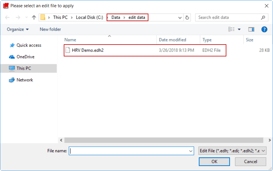
Edit files created in HRV 3.2 have the file extension “.edh2″. They are by default stored in a subdirectory of the data files directory called edit data, but can be stored anywhere you choose.
User Preferences
These files are created automatically when either:
- The data file is created in BioLab or
- The data file is opened in a MindWare analysis application
They follow the naming convention:
Data File Name_userpreferences.cfg
and are stored in the same directory as the data file.
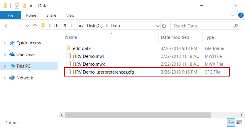
As long as these files are stored in the same directory as their corresponding data file, certain file-specific settings will be preserved between uses of the application and when the file is opened in other analysis applications.
Configuration
The analysis applications contain many configurable settings, and these settings may vary between studies, files, or subjects. When multiple researchers are using the application concurrently, or when you simply want to backup your settings for peace of mind, saving a configuration file is the way to do it. These files can then be loaded to restore settings to a known state before proceeding with analysis. Configuration files have the “.hrvcfg2” file extension.
Output
Statistics derived from analysis can be written out to a file for use in higher level statistical analysis packages. The output is stored in Excel (.xlsx) format.
Channels & Signals
Data files consist of multiple channels, each of which was used to acquire a particular signal. In the analysis application, you will have to map each of these channels to a signal type, which will dictate how the application uses them. Throughout the guide/application, these terms are used interchangeably to describe the same thing.
Events
Events are specific points of interest in a data file. You may want to base your data analysis procedures on these events (for example, when these events indicate the start/end of a particular task), or they may just be for reference to explain a change in physiology/subject behavior. These are most commonly created during data collection but are sometimes generated post-acquisition depending on your workflow/tools used.
Event Sources
Events can come from a variety of sources. They may be stored as special time points in the data file itself, derived from a channel, or read from an auxiliary file from another system used during data acquisition. The specific event sources that are supported in the application will be discussed in more detail later.
Segments
Data files are divided into segments for analysis purposes. These segments can be defined in logical ways based on your experimental protocol using either time or events. At any given time, only a single segment is visible on the analysis screen.
Launching the Application
To launch the HRV application, double-click the shortcut on your desktop
![]()
Or navigate to the MindWare folder from the Start menu and select HRV Analysis 3.2
Be sure to insert your software key before launching the application!
A quick note on licensing
MindWare applications are licensed through the use of a Software Key, the small silver USB key that you received with the purchase of the software.
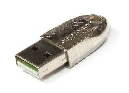
These keys can hold the license to multiple applications, or to a single application, depending on how the software was purchased. To view which licenses are on your software key, you can use the License Manager.
A software key with a license to run HRV 3.2 must remain plugged into the computer throughout the use of the application. If the software key is not detected, you will receive an error message:

The options at this point are to insert the software key, exit the application, or proceed in Demo Mode. Which brings us to our next quick aside…
A quick note on Demo Mode
If you have just downloaded the application to try it out – welcome, and thank you for taking the time to evaluate this application! You don’t need a software key to unlock the full capabilities of the software for evaluation purposes, with one caveat – it will only work with specific demonstration files.
Some demo files are automatically installed with the application, and when in Demo Mode, the demo data folder (My Documents/MindWare/HRV Examples) will automatically open when prompted to select a file. You can also go to Help>>Download Demo Data… on the Setup screen to download additional example files.
When you find you can no longer survive without this application aiding you in your research endeavors, feel free to visit our online store or contact a MindWare sales representative ([email protected]) to purchase a full license.
Selecting a file for analysis
Once the application is running, the first thing to do is to select a data file for analysis.
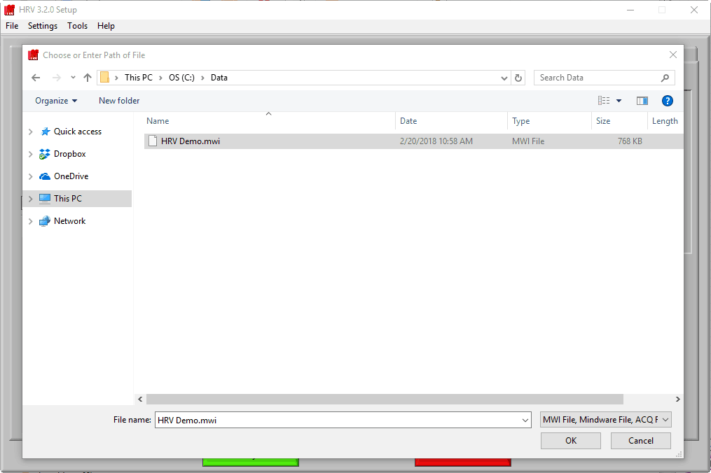
Navigate to the data file of your choosing, and either double-click it or highlight it and press OK. Many popular data file types are supported:
.mwx/.mwi
This is the file type that is written by Mindware BioLab 3.1 and newer. The applications are designed to work seamlessly with this file format and there are many advantages to using these files:
- Data is automatically scaled to the appropriate units, when possible
- Events are stored directly in the file (we’ll cover this more in a bit)
- Video files recorded in BioLab are automatically selected for use
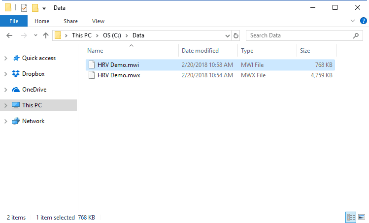
Note that when working with these files, the “.mwi” is opened from the file dialog, but both are required for analysis and must be stored in the same directory.
.mw
This is the file type that was written by MindWare BioLab 3.0 and earlier. These files lack some of the additional information stored in MWX/MWI files.
.acq
These are BioPac AcqKnowledge data files. They must be stored as a “Windows AcqKnowledge 3 Graph” before being used for analysis.
.edf
This is the European Data Format, a popular open source file format. Visit the official website for more information on this file format.
.bdf
This is the BioSemi data format, an offshoot of the EDF file format but used exclusively by BioSemi acquisition hardware.
IBI.txt
The HRV application also allows opening a text file which contains a series of inter-beat interval (IBI) values, also referred to as heart period, R-R period, or beat-to-beat period. When opening an IBI text file, the IBI Import Wizard will launch.
IBI Import Wizard
Not all IBI files are created equal, and there is no standard format for their storage across different devices. The IBI Import Wizard allows you to define how your IBI data is stored so that it can be correctly loaded for analysis.
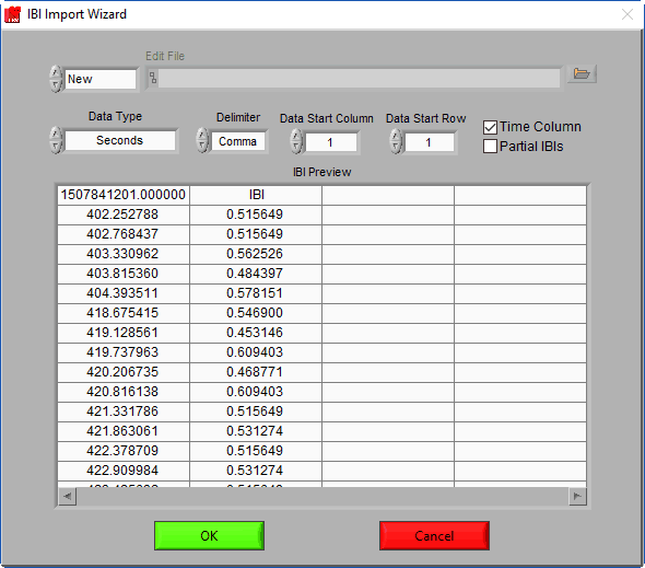
There are several settings available:
Data Type
IBIs can be specified in either (fractional) seconds or milliseconds
Delimiter
If there are multiple columns in your IBI file, they can be separated by tab, space, or comma characters.
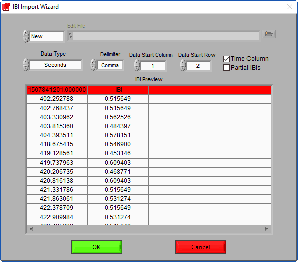
Data Start Column/Row
If there is header information or additional channels in the IBI file, these settings are used to ignore them. Adjust these values so that the start row and column correspond to the start of the IBI series.
Time Column
Check this box if the first column in the IBI file represents relative time from the start of data acquisition. This will be used to better display the IBI values during analysis.
Partial IBIs
Indicates if the first/last IBIs are partial, based on the start/end of data acquisition.
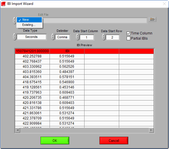
Edit File
That’s right – you can edit an IBI series too! Selecting an edit file will automatically configure the IBI Import Wizard to import the data the same way as it was when the editing took place. To open an edit file, change the mode from New to Existing and select the desired edit file.
Other
Even if your data file is not on this list, there is a good chance you can still analyze it! Check out this article on the ASCII-MW converter for more information.
Want to see your preferred file format read directly? Let us know!
Channel Mapping
After selecting a data file for analysis, the application will prompt you to map the channels to the signal types that the application will use.
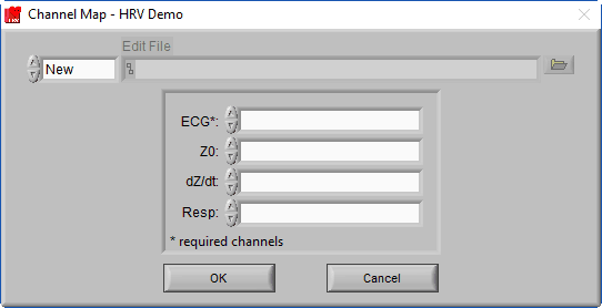
Recall that a channel is simply a container in the data file for a particular signal, but at this point, the precise signal type is unknown to the HRV application. Ideally, the channel has been named such that it is obvious what signal type it contains, so this step should be easy.

The HRV application uses ECG and respiration signals to derive all of the relevant statistics. Only ECG is required (denoted by a * next to the signal type), but respiration is highly encouraged as it is used to validate high-frequency HRV statistics.
Respiration can be measured directly (through use of an instrument such as a respiration belt) or it can be derived from either of the cardiac impedance signals, Z0 and dZ/dt. You will specify which of these channels you want to use for respiration later, but for now, simply map each channel to the corresponding signal type.
Edit Files
We aren’t quite done with the Channel Mapping screen yet. This is also where you will specify the edit file you intend to load.
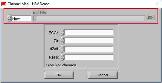
When a data file is opened for the first time, the edit file will default to New, since no edits exist yet for this dataset. Once a dataset is edited and opened for the second time, the last used edit file will automatically be loaded.
When an edit file is loaded, you will notice that the channel mapping is done for you, set the way it was when the edit file was created.
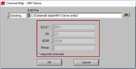
This is because the channel mapping is stored in the edit file, and automatically applied to ensure the edits are applied to the correct channels in the file. There are a few other settings which will also be affected in this way, which we will cover a little later.
If you wish to open a different edit file, click the browse button next to the Edit File path
![]()
To start a new edit file from scratch, make sure the mode is set to New
![]()
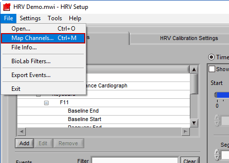
Modifying the channel map
If you have multiple subjects’ data stored in a single file, if you want to load a new edit file, or if you made a mistake in your original channel mapping, you can always change it by going to File>>Map Channels… or use the hotkey Ctrl+M on the Setup screen.
Setup Screen
The setup screen is where everything in the application is configured, including the way the data is segmented, specific algorithm settings, video playback settings, and much more.
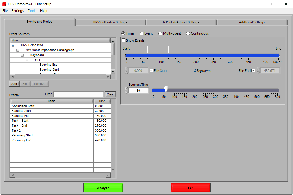
Some of these settings are available across all MindWare analysis applications, so they may look familiar. Others are specific to the HRV application. This section of the guide will cover all of these options in detail, starting with Events and Modes.
Events & Modes
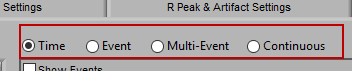
As mentioned earlier, data analysis is always performed in segments – portions of time defined either by specific time intervals or by events. The way the data is segmented during analysis can have a significant impact on the results, and segmentation must be considered carefully before proceeding with analysis. The settings on the Events & Modes tab are used to define these segments. There are four main modes available in HRV 3.2, which are selected from the mode selector:
Let’s start by examining the left of the screen, where there are two lists – Event Sources and Events.
Event Sources

Event sources represent all available events that could occur within a data file. They are displayed in a hierarchical manner, and it is common (especially when using MWX/MWI files) to see nested event sources, which help give further clarity to the origin and meaning of an event. It is possible to use both Event Sources and Events to define data segments.
Note: These lists represent all available event sources and events, but they do not all necessarily need to be used for analysis. We will talk about how to use these later.
Now let’s go over how Event Sources are loaded into the application.
Default Event Sources
By default, any event sources that are stored within the currently opened data file will automatically populate in the event sources list. You can tell an event source is default a couple of ways:
- It cannot be removed from the list:
- The first level in the event source hierarchy is the name of the data file opened:
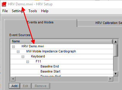
Note: Currently, only MWX/MWI files and ACQ files are supported as defaults
Adding an Event Source
To add an event source, press the Add button below the Event Sources list:
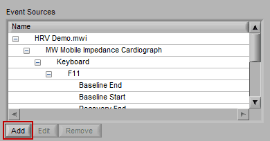
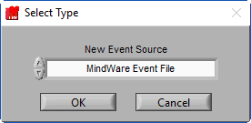
A new window will appear, prompting you to select the type of event source you would like to add:
Note: You will typically only have a couple of these, but you can add as many as you require
There are several types of event sources supported:
MindWare Event File
The MindWare Event file is a text-based format used by BioLab 3.0 and earlier. It is also quite useful as an intermediary file format to bring external events into the analysis applications.
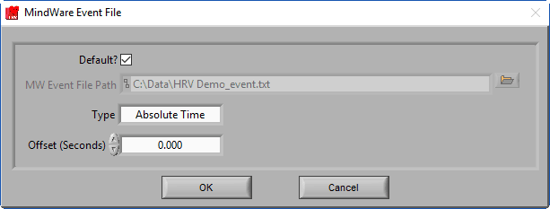
If a properly named MindWare Event file is identified, it will automatically populate the file path and select the Default? option. A properly named MW event file uses the following naming convention:
Data file name minus extension_event.txt
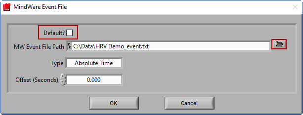
And is stored in the same directory as the data file. Versions of BioLab that wrote this event file (3.0 and earlier) name the files this way automatically, but if you are using the MW Event file format to bring in events from an unsupported 3rd party system, make sure you name them well to be automatically identified. Otherwise, ensure Default? Is unchecked and press the Browse button to select a file with a different naming convention.
There are two types of MindWare event files – Absolute Time and Relative Time. Absolute Time is based on the actual wall clock time of the event and Relative Time is based on time elapsed from the start of the acquisition. Depending on the way the events are stored in the file, the Type will need to be updated accordingly.
You also have the option of offsetting events in the file by a specific time constant (in fractional seconds).

This is particularly useful for bringing in events from a 3rd party system which was not started in sync with physiology data collection.
If you attempt to open a MindWare Event file that is not properly formatted, you will receive an error.
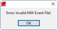
If this happens, check your event file and try again.
Noldus Observation File
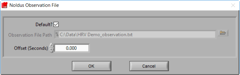
MindWare applications support integration with Noldus Observer XT during both data acquisition and analysis. Once an observation has been completed, you can bring the observation data (in .txt format) into the analysis applications via a Noldus Observation file. This type of event source behaves in the same way as a MindWare Event file, but with a slightly different default naming convention:
Data file name minus extension_observation.txt
For more information on exporting these observations from Noldus Observer, see this article.
Digital Event Channel

Events can also be derived from channels within the data file. Most commonly, these channels represent either individual digital lines used to capture event markers from integrated systems during data collection, or a summary representation of a group of these digital lines. When detecting events from a channel such as this, the application is looking for changes in the value of the channel that are maintained for some duration of time.
The following settings are available, and should be set based on the system used to generate the digital events:
- Channel name – the channel on which to search for events
- Pulse direction – look for changes in the positive direction, the negative direction, or both
- Pulse width – how long a change needs to persist in the channel before it is considered an event. This can help prevent multiple events from being detected when there is noise in the digital line
Note: In BioLab 3.0 and greater, digital events are also stored as events in the data file (or event file) and therefore it is not necessary to load them this way.
Editing an Event Source
To edit the details of an event source, highlight any item within the hierarchy and press Edit.
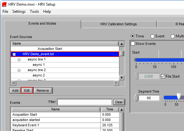
Note: Default event sources cannot be edited
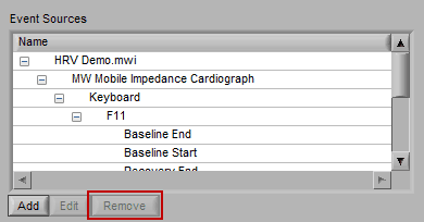
Removing an Event Source
Much like editing event sources, to delete simply highlight any item in the hierarchy and press Remove
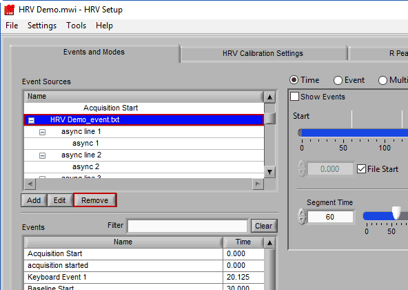
Note: Default event sources cannot be removed. Also keep in mind that even though an event source is listed here, that does not necessarily mean it is being used for analysis.
Some caveats on how event sources are loaded
First, any default event sources will be loaded. Next, if any event sources are stored in the User Preferences file, those will be loaded. These event sources reflect those chosen the last time the file was analyzed. If there are no event sources in the User Preferences file, the application will try to load whatever event sources were used with the last data file that was opened. If these event sources are not available for the current data file, you will receive a warning stating such:
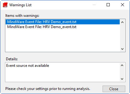
Event sources which are dependent on the data file name (such as MW Event and Noldus Observation files) will automatically update to search for the current data file default path. If you are not using the default naming convention for these files, you will need to specify them for each new data file you analyze.
Events

Events are the specific instances of event sources, occurring at a given time. The event list consists of pairs of an event source name and the time at which it occurred. Events can be selected by left-clicking them. Select multiple events by Ctrl+click. Select a range of events by selecting the first event, and then Shift+click the last event.
Filtering the event list
When an event list is large, it may be useful to filter the list by the event name to isolate the events of interest. There are a few ways you can do this:
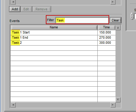
Manual Entry
Begin typing the desired event name into the Filter box, and the events which qualify will remain visible in the list:
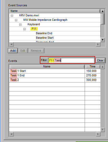
Specific events in the event source hierarchy can be filtered directly by separating the levels of the hierarchy with the “:” character, as shown in this example:
Drag and drop Event
To find all occurrences of a specific event, left-click it in the events list and, while holding the mouse button, begin to drag it. You will notice how the Filter text box is highlighted, and the selected event is floating outside the list:
Drag the event into the Filter box, at which point it will turn green to indicate it is ready to be dropped:
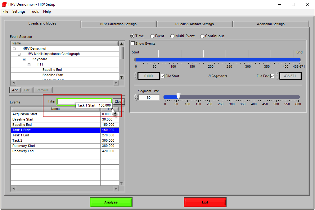
Release the left click to automatically filter based on that event:

Drag and Drop Event Source
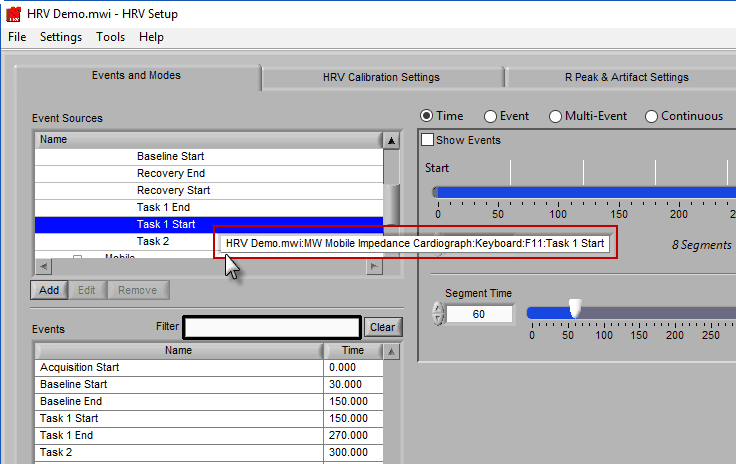
The same action can be done on an event source at any level in the hierarchy. When this is done, events will be filtered both by name and source:
Time Mode
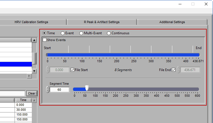
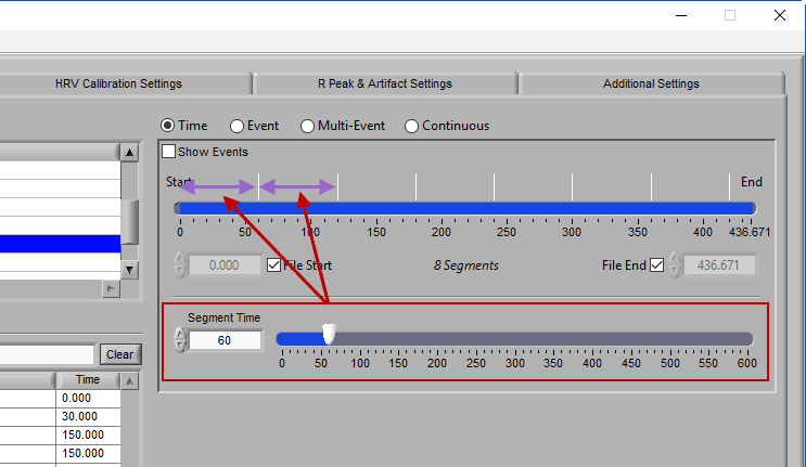
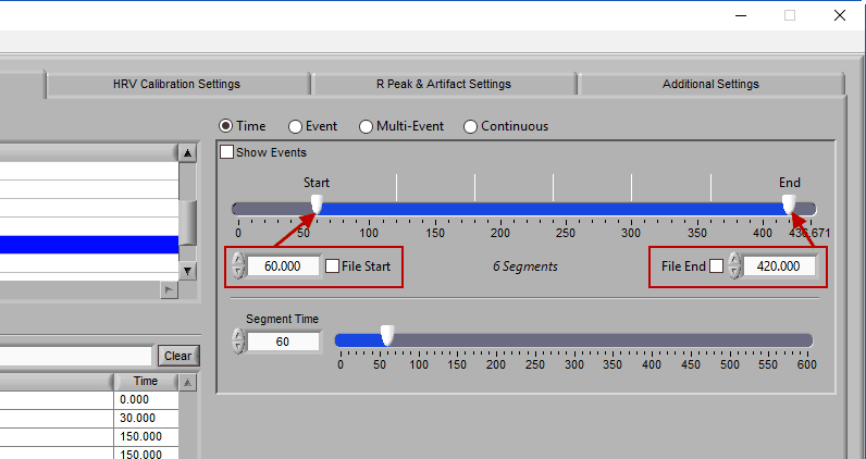
Time mode is used for (you guessed it) segmenting your data in fixed time intervals. The timeline indicates the currently selected start and end time for analysis. Individual segments are notated with grey lines along the timeline, the duration of which is defined by Segment Time.
To modify the start/end time of analysis, uncheck File Start or File End and drag the start/end point to the desired time (or manually input a start or end time):
Using events in Time mode
There are some opportunities to use events to assist in analyzing the data in Time mode, even if the segments aren’t defined directly by them. First, there is an option to Show Events:
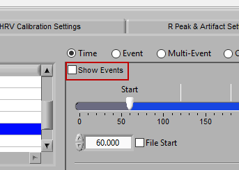
When this is checked, events will be shown in the data segments as they occur, which can be useful for reference when determining the cause of physiologic changes or noise in the data.
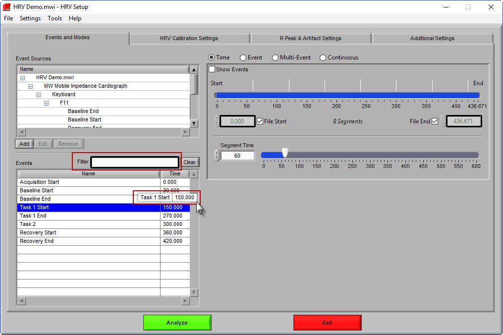
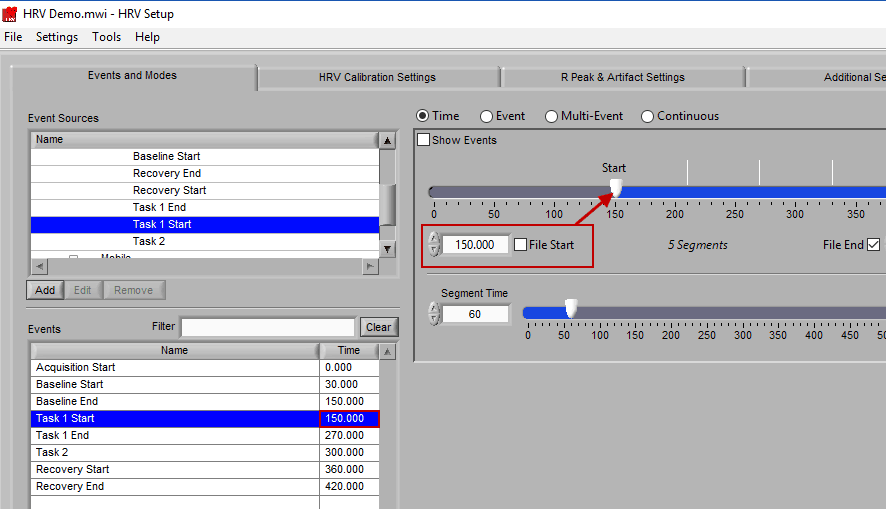
The second way events can be used is to help define a start and end time for analysis. To start/end analysis at a certain event, left-click that event in the Events list and drag it into the Start Time or End Time field.
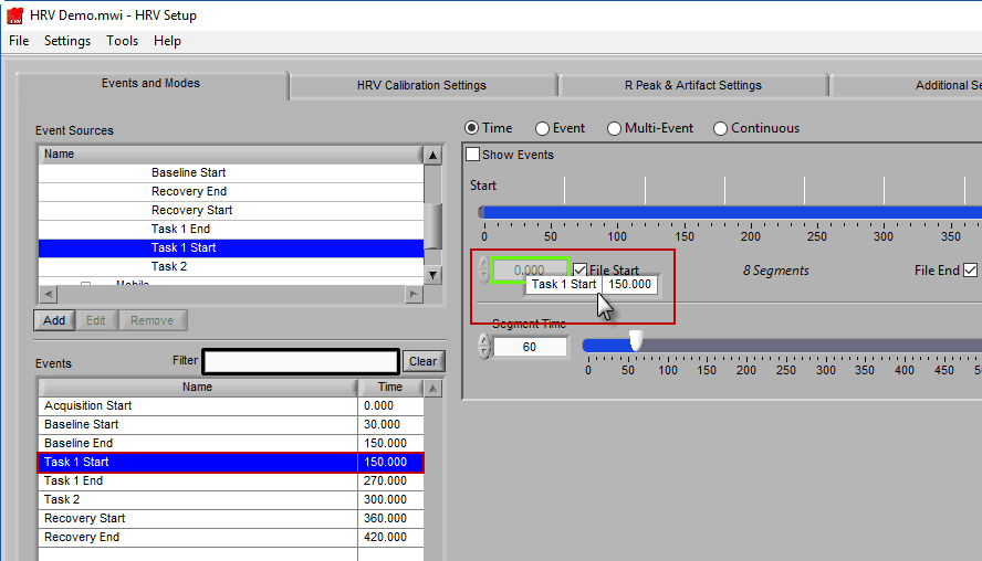
This will automatically adjust the start/end time to that event time.
If you are interested in learning other, more powerful ways to use events, continue on to the next section on Event mode.
Event Mode
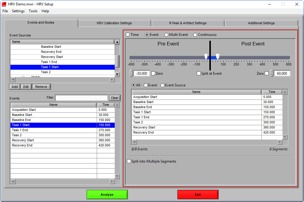
Event mode allows you to use pre-defined, specifically labeled time points in the data file to define your segmentation. Use of events can be very powerful for data analysis and can be a serious time saver over constantly adjusting Time mode settings to view specific time points of interest. These events are typically stored during data acquisition, but can also be entered post-acquisition using applications such as BioLab.
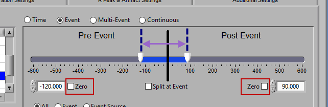
Using the timeline
At the top is the segment timeline, but rather than being based on the start and end of the data file, it is now based on the occurrence of an event, indicated by the black vertical line in the timeline:
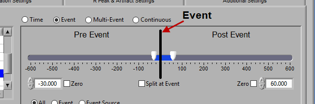
The two sliders on the timeline can be dragged on either side of the event, and frame what time around the event is of interest:
There are many different ways you can view your data using the timeline.
Pre Event
To look strictly pre-event, lock the end slider to the event by checking Zero next to the end time and drag the start slider to the left of the event, or enter a time manually. Keep in mind that since we are looking at the time relative to an event, the start time will be a negative number.
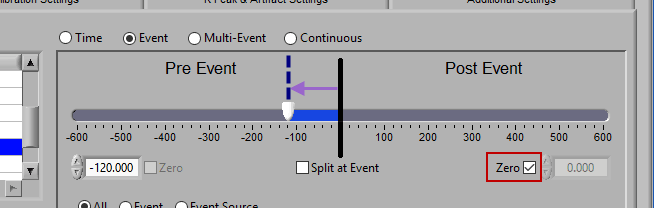
Post Event
Similarly, lock the start slider to the event by checking Zero next to the start time and drag the end slider to the right of the event, or enter a time manually to look strictly post-event.

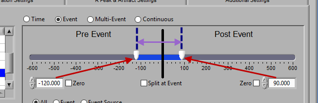
Pre and Post Event (single segment)
To look at some amount of time before and after each event in a single segment, make sure both sliders aren’t locked to the event and drag them where you desire on either side of the event.
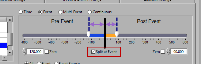
Pre and Post Event (multiple segments)
To look at pre and post-event times in their own segments, check the Split at Event option. This will cause the pre and post event portions of the timeline to appear different colors.
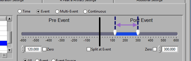
Segment based on, but not including an event
To look at a segment that is based on the time of an event, but does not include the actual event, drag both sliders to either side of the event in the timeline.
Events to Use
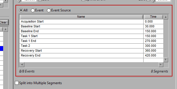
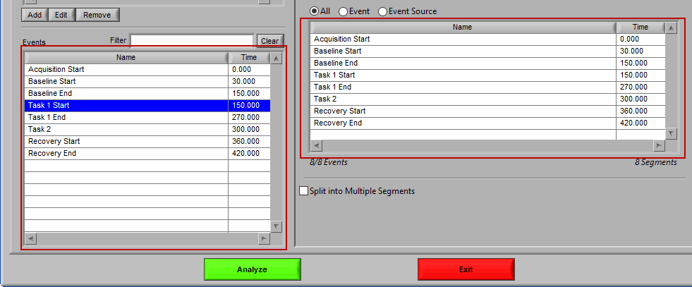
As mentioned earlier, just because an Event Source/Event is listed to the left does not mean it will be used for analysis. Rather, they must be selected from that list explicitly. There are 3 ways events can be selected: All, Event, and Event Source.
All
All events in the event list will be used for analysis:
Event
Use event-based selection when there are specific instances of events that you want to analyze based on. Any of the events in the Events list can be selected for use. Ctrl-click to select multiple events, and Shift-click to select a range of events.
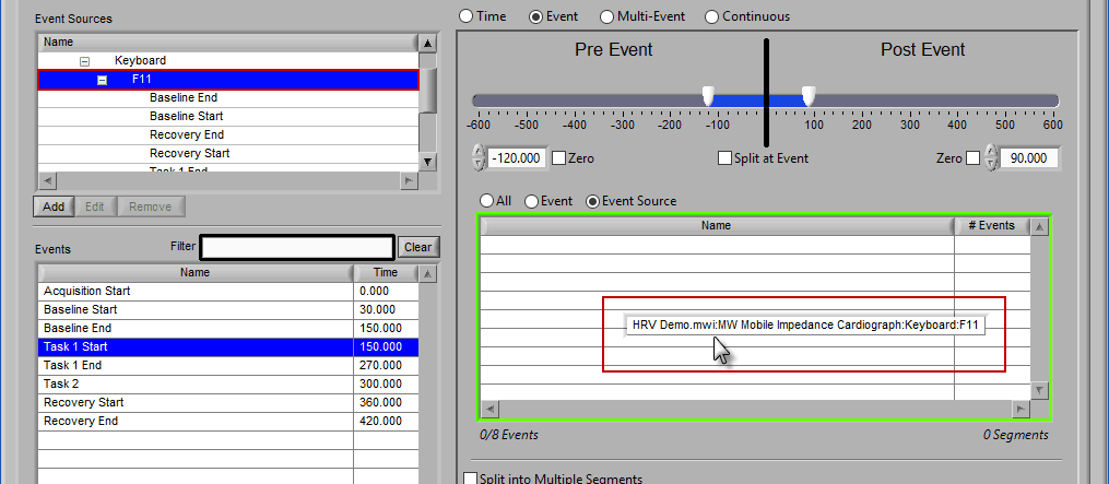
Adding Events to Use
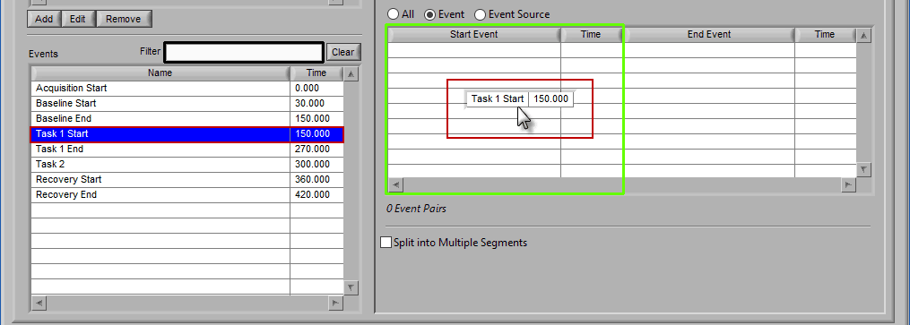
To add events to this list, drag and drop events from the Events list into the Events to Use list. This is done by left-clicking on the desired events in the Events list and dragging those events out of that list and into the Events to Use list.
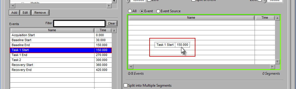
When the Events to Use list is highlighted in green, that means the event can be dropped. Release the mouse button to add the event to the list.
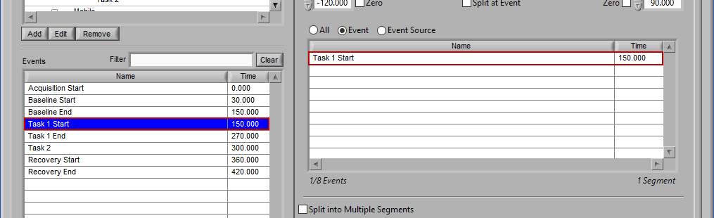
Events will be sorted in chronological order automatically as they are added to the list.
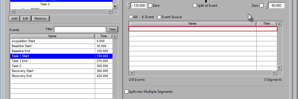
Removing Events to Use
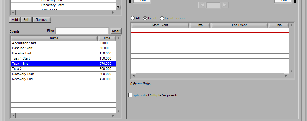
To remove events from this list, select the event(s) to remove and drag them anywhere outside of the Events to Use list. The list will be highlighted red to indicate events will be removed.

Release the mouse button to remove the event from the list:
Event Source
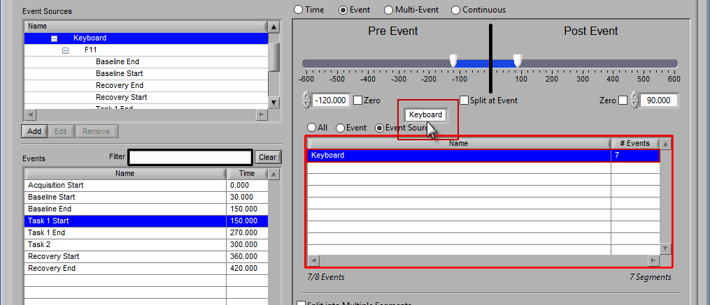
The same can be done for event sources. When analyzing based on a source, all instances of a given event source will automatically be used for analysis. The right-most column in the list indicates how many instances of that source will be used.

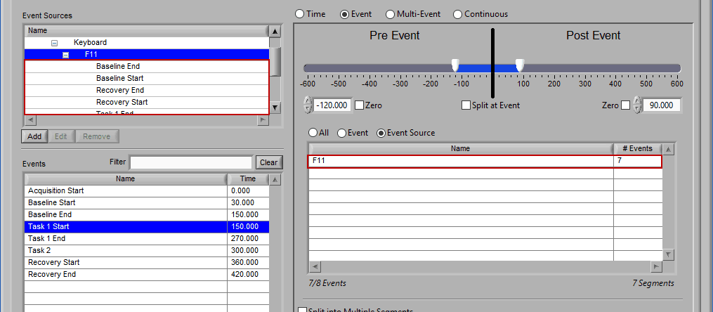
Adding Event Sources to Use
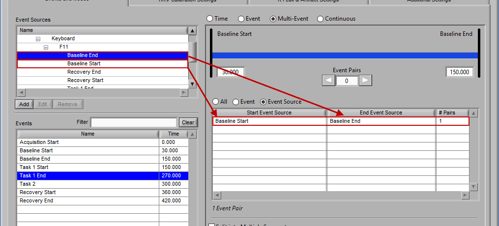
Similar to Event-based selection, drag and drop event sources from the list on the left to use them for analysis:
Notice how the F11 event source contains multiple events, indicated by the rightmost column in the table.
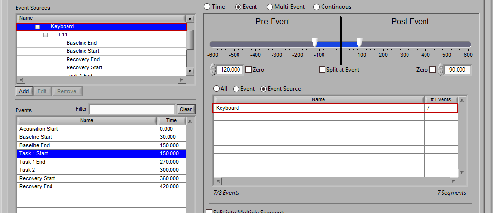
If an event source at a higher level in the hierarchy is chosen, all occurrences of event sources below it will also be selected for analysis:
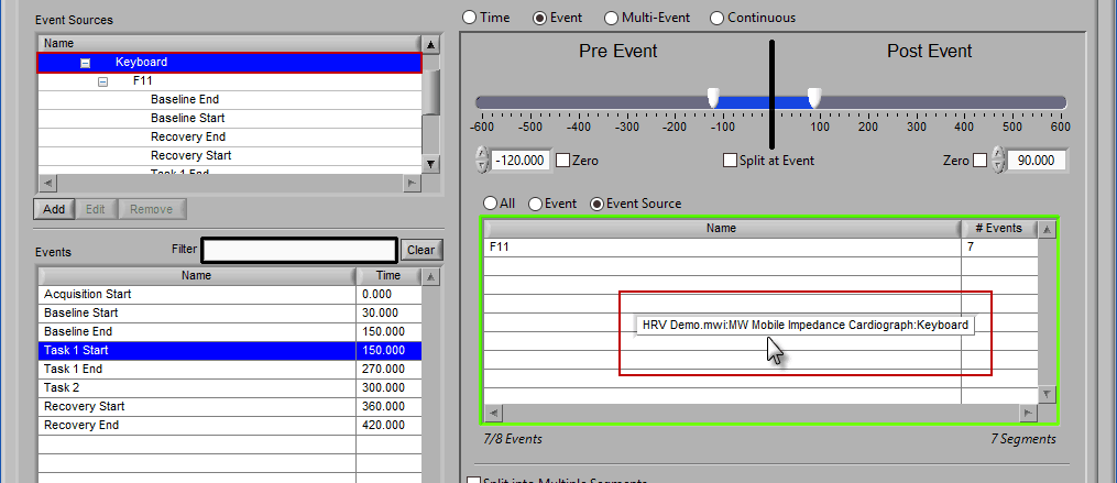
Any entries which were already in the event sources to use list will be replaced by the higher level event source.
Removing Event Sources to Use
This is done the same way as removing an event from the list – select the event source(s) to remove, drag the selection outside of the list,
and releasing the mouse button to remove from the list.

Switching between selection modes
When switching between the selection modes, it is possible to preserve the events currently selected for use in the new mode:
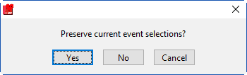
When events selections are preserved, the new selection mode will already contain the events used in the previous mode. If events are not preserved, the list will be empty in the new mode.
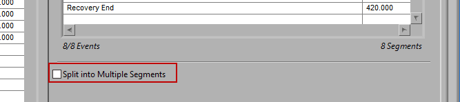
Split into Segments
It is best practice to only analyze your data in as big of segments as are absolutely necessary to obtain the desired statistics. If a large amount of data around a given event is pertinent to your study, it may become unmanageable to edit all at once. By checking Split into Segments, you can divide the specified timeline into smaller segments for more convenient analysis.
When this is selected, the grey lines on the timeline indicate the segments. Adjust the Segment Time to change the amount of time per segment.
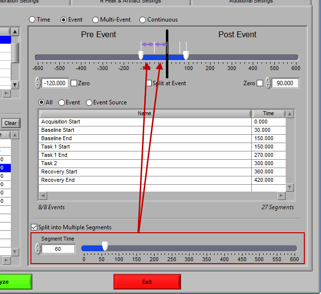
It is possible to have partial segments if the total time is not evenly divisible by the segment time (as evident in the image above).
Multi-Event Mode

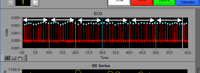
Multi-event mode allows you to specify a segment between two events. This is particularly useful if you use events to indicate the start and end of epochs in your study. The timeline is again present at the top, but event lines exist at either end. The names and times of each event are located next to the event line:
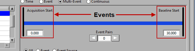
Use the left and right arrows to preview the segments which will be created from the selected events:
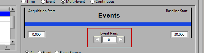
This is particularly useful when using Event Sources to define multi-event segments, since not all events being used will be obvious.
Events to Use
This section works very similarly to Event mode, except that each segment requires the selection of 2 events rather than one – a start event and an end event.
Again, there are 3 ways to select events – All, Event, or Event Source.
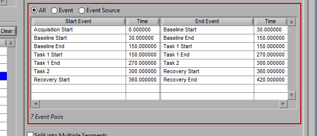
All
All events will be used for analysis. First event in file -> second event, second event -> third event, etc.
Event
When selecting by event, each segment is defined by two events.
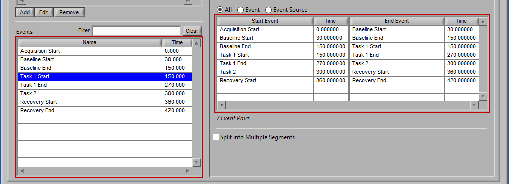
Adding Events to Use
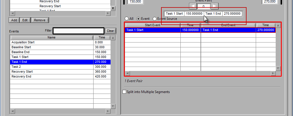
The start event will always be selected before the end event. To select the start event, drag and drop an event from the list. Notice how the column which contains the Start Event is highlighted green, ready to accept the event.
Once a start event has been selected, drag the second event into the list to set it as the end event.

Removing Events to Use
Events are removed from the list in pairs. Select the desired pair(s), drag out of the list:
And release the mouse button to remove from the list.
Event Source
Adding and removing event sources uses the same drag and drop principles as events, except items are selected from the Event Sources list:
Notice the list contains a # Pairs column. Since we are using event sources, and each of which could contain one or more event occurrences, there may be more than one possible segment between the start and end event sources. Let’s take the F11 event source as an example, which contains many event sources beneath it.
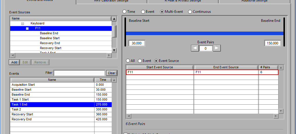
This is essentially saying “create segments from any subsequent occurrences of an F11 event”. In this file, there 7 events which fall under the F11 event source, so there will be a total of 6 segments created. This is where scrolling through event pairs becomes useful since the events themselves are not clearly listed in the Event Sources to Use list.
Split into Segments
Much like event mode, these multi-event segments can be further broken into smaller segments by checking Split into Multiple Segments
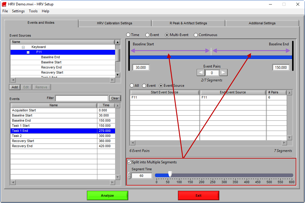
Again, segments are indicated by grey vertical lines on the timeline, and it is possible to have partial segments if the time between events is not evenly divisible by the Segment Time.
Continuous
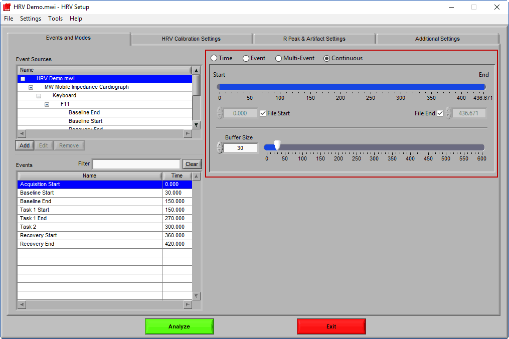
Continuous mode is specific to the HRV application and allows you to calculate second-by-second statistics using a moving fixed width buffer.
Much like Time mode, the timeline is used to define the start and end points of analysis. Events can be dragged from the Event list to set the start and end time as well. Buffer Size defines the size of the moving window from which statistics are calculated.
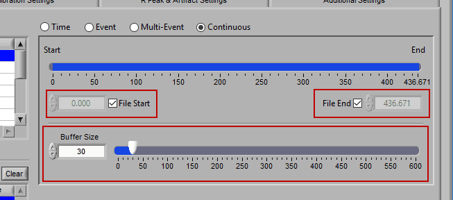
Note: At least a 30 second buffer is required to calculate RSA and frequency-based statistics.
Analysis is performed by starting at the start time with a segment of data equal to the buffer size. Statistics are then calculated on this segment. Next, the start/end of the segment are incremented by 1 second, statistics are calculated, and so on until the end of the segment reaches the specified end time.
HRV Calibration Settings
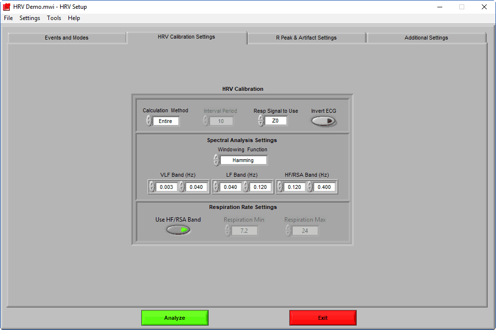
The HRV Calibration settings page contains settings which are specific to the HRV application and the algorithms used to obtain important statistics. The algorithms themselves will only be covered in as much detail as is required to describe these settings. If you are interested in learning more, please visit our blog.
Calculation Method
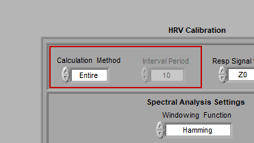
Interval mode allows you to further break down each segment into smaller intervals. Only a few statistics are calculated for each interval:
- Heart Rate
- Mean IBI
- # R Peaks
This can be very useful if you are interested in second by second heart rate, but still want to study RSA. To do this, select Interval mode with an Interval Time of 1 second:

Respiration Signal to Use
Remember on the channel mapping screen, where you were asked to identify both cardiac impedance channels and/or a respiration channel? This is where you specify which of those channels are actually used for respiration.
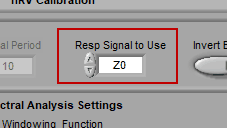
Respiration channels are used directly, without any additional processing. Cardiac impedance channels must be processed to isolate the respiratory content.
Note: Automatically set and disabled when using edit files
Invert ECG
ECG can be inverted when the positive and negative electrodes are swapped during data collection. If this happened, don’t worry about it – we can easily invert the signal in the application by pressing the Invert ECG button.
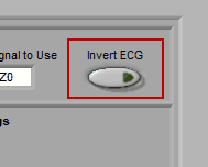
Not sure if your ECG is inverted? There is also a way to invert the signal on the analysis screen, so you can have a look before making a decision.
Note: Automatically set and disabled when using edit files
Spectral Settings
Spectral settings pertain to the bands which define the three main frequency ranges of interest for heart rate variability – Very Low Frequency (VLF), Low Frequency (LF), and High Frequency/RSA (HF/RSA).
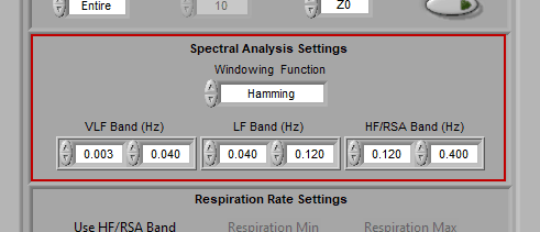
The frequency ranges used may vary based on age and species of subject.
Note: Frequency bands cannot overlap.
The window is typically set to Hamming, but many spectral windows are available for use.
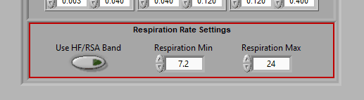
Respiration Rate Settings
By default, respiration rate is identified by looking for the peak frequency in the HF/RSA frequency band.
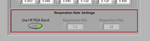
This is because the respiration must occur in this band to validate RSA. If you are not interested in RSA and wish to identify respiration rates outside of the typical band, disable Use HF/RSA Band and use the Respiration Min/Max to set the range of interest (in breaths per minute).
R Peak & Artifact Settings
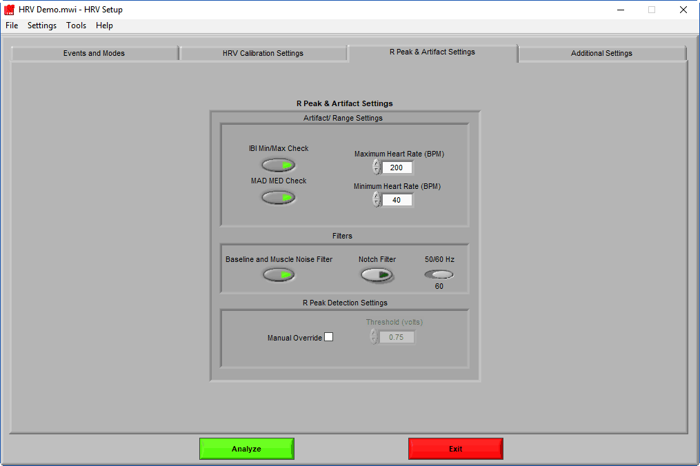
A key component of HRV analysis is identifying the R peak of the ECG signal, and being able to differentiate between a good peak and potential artifact. On this tab, the algorithms responsible for doing just that can be tweaked for your specific data set/population.
Artifact/Range Settings
There are two types of artifact detection algorithms available: IBI Min/Max and MAD/MED.
IBI Min/Max
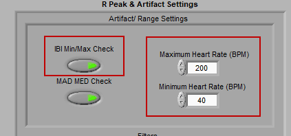
This algorithm simply checks if an inter-beat interval falls above or below the specified heart rate thresholds. If it does, the beat will be flagged as a potential artifact. By default, these values are set at 200 BPM and 40 BPM, but can be adjusted to account for the desired range.
MAD/MED

The MAD/MED algorithm places some bounds on the variability of the inter-beat interval from beat to beat, and flags beats which exceed these limits. The details of the algorithm can be found here.
Filters
Note: Filters are automatically set and disabled when using edit files
There are two filters which can be applied to the ECG signal. The first is a Baseline and Muscle Noise filter, which is a bandpass filter between 0.5 Hz and 45 Hz. This filter helps to isolate the frequency components that are most commonly associated with ECG.
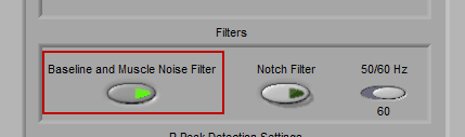
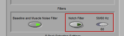
The second filter is a Notch filter designed to remove interference from electrical components that may have affected data collected. Most electricity around the world runs at either 50 or 60 Hz, so it is possible to select one or the other, whichever is appropriate for the locale where the data was collected.
BioLab Filter
In addition to the two filters available on the R Peak & Artifact Settings, it is possible to apply the filter(s) used during data acquisition in BioLab. To view/enable these filters, go to File>>BioLab Filters…

From this screen, you can view the filters which were used during acquisition, and apply them to each channel by pressing the Use BioLab Filters button
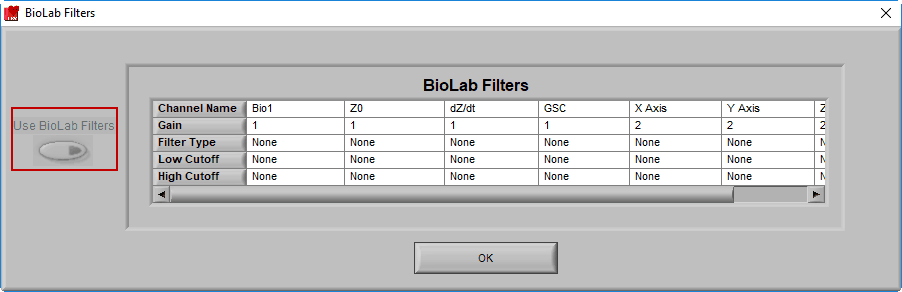
Note: This option will be disabled if no BioLab filters are available, or if you are using a data file type that wasn’t created by BioLab, or if you are using an edit file
R Peak Detection Settings
By default, R peaks will be detected using the Shannon Energy Envelope technique. In some cases, particularly when an ECG signal is abnormal or you have mapped a different signal than ECG, a simple threshold detection will work better than this technique. Enable Manual Override to use threshold detection, and adjust the threshold accordingly.

Additional Settings
Like the Events and Modes section, these settings will be available in all MindWare analysis applications.
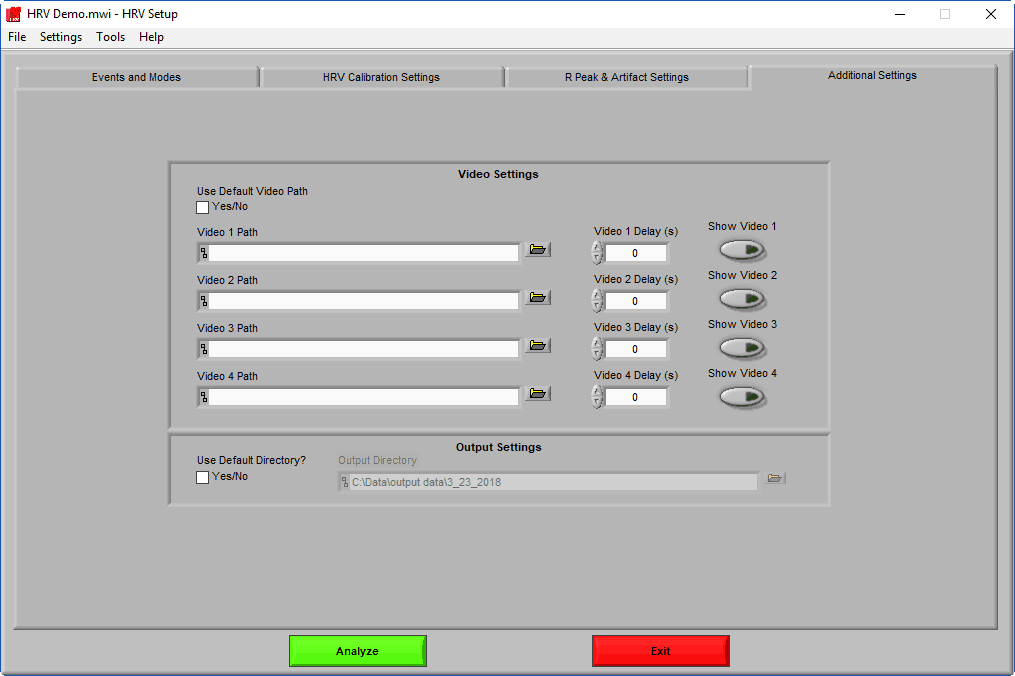
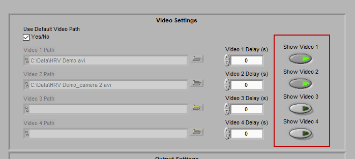
Video Settings
Up to 4 videos can be loaded for playback during data analysis. Viewing video can provide great insights into subject behavior and can be helpful in identifying the source of artifact in the data. Videos must be in either AVI or MPEG format. If your videos are in a different format, you can most likely find a converter online to translate them to one of these two formats.
Selecting videos for playback
When “Use Default Video Path” is selected, the application will automatically search for video files in the same directory as the data file which adhere to this naming convention:
Data-File-Name.mpg
Data-File-Name_camera 2.mpg
…
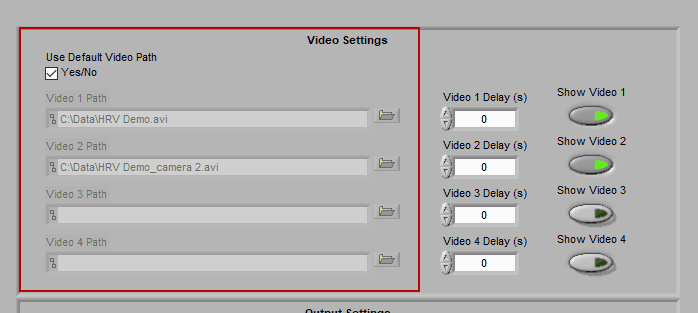
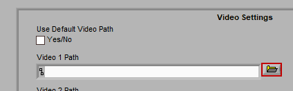
Videos collected in BioLab will automatically be named correctly and stored in the proper location. If you have moved/renamed your videos, or collected them using a different system, you will have to identify them manually. To do this, press the Browse button next to each video path and navigate to the desired video.
Using video delay
The start of video playback can be aligned to the start of the data file by setting a video delay
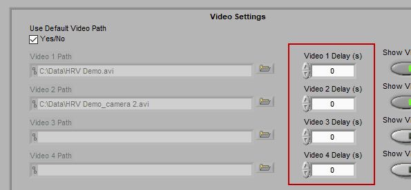
This is useful for when videos were collected with a separate application than the data file and the two applications were not started simultaneously. If the videos started before the data file, use a negative delay, and vice versa.
A note for Noldus Media Recorder users
If you are using Noldus Media Recorder in conjunction with BioLab to record your videos, you can restore the “default” video delay calculated at the time of acquisition by right-clicking the delay field and selecting Reset.

Enabling a video for playback
Make sure to press “Show Video” for each video you wish to view during analysis.
Output Settings
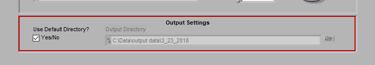
By default, the output file is stored in the subdirectory
/Output Files/Current Date
of the same directory where the data file is stored.
If you would like to store your output files in a different directory by default, uncheck Use Default Directory? and modify the path as you see fit. You can always change the name and location of the output file when it is created during analysis as well.
Using Configuration Files
As mentioned in the first section, configuration files are a great way to backup your current settings or ensure that the application is configured exactly as you expect it to be.
Opening a Configuration File
To open a configuration file, go to Settings>>Open Configuration… and select a “.hrvcfg2” configuration file.
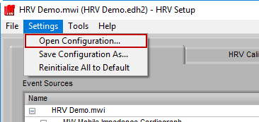
Note: Opening a configuration file will override all current settings with those stored in the configuration file
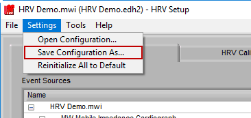
Saving a Configuration File
To save a configuration file, go to Settings>>Save Configuration As…
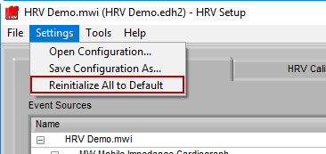
Reinitialize All to Default
To start from scratch, go to Settings>>Reinitialize All to Default. This will clear all current settings, so be careful to not do this unless you intend to!
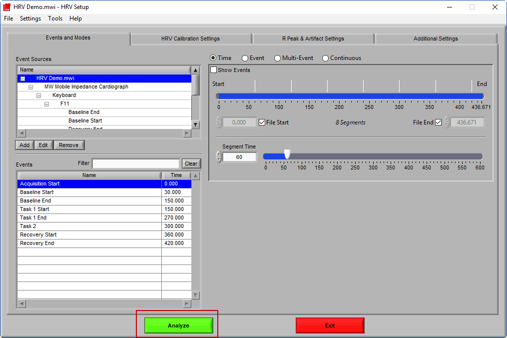
Proceeding to Analysis
To start data analysis, press the Analyze button:
Analysis Screen
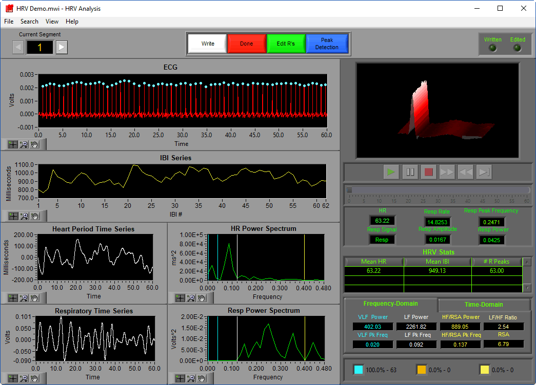
The analysis screen is where data is viewed, transformed, and processed to produce statistics related to Heart Rate Variability.
Data Graphs
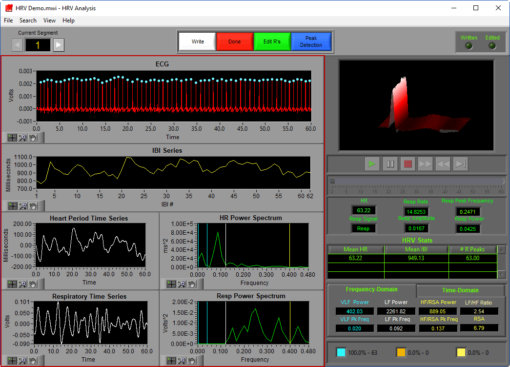
In this portion of the analysis screen, signals from the data file for the current segment are shown in various stages of processing. It is from these signals that all statistics are calculated.
Each graph has a set of graph tools, which can be used to zoom into and move through the data in finer detail. These tools are found in the lower left-hand corner of each graph. See this article for more information on how to use these tools.
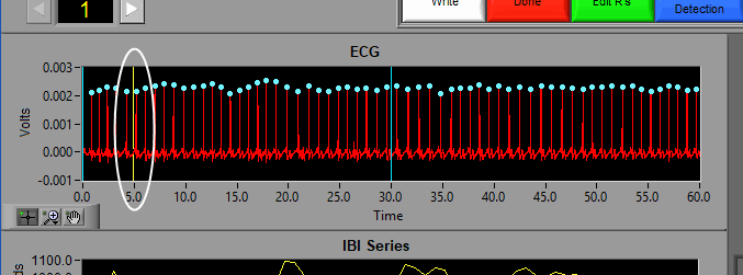
ECG
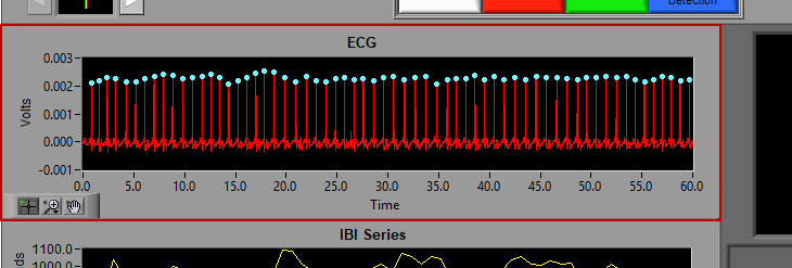
The ECG graph shows the channel mapped as ECG in red. You will notice the detected R peaks on the signal are marked with (potentially) a few different colors. A blue dot indicates an R peak with has passed the artifact detection algorithms:

A yellow dot indicates one or more of the artifact detection algorithms has flagged this peak as potential artifact and requires further inspection:
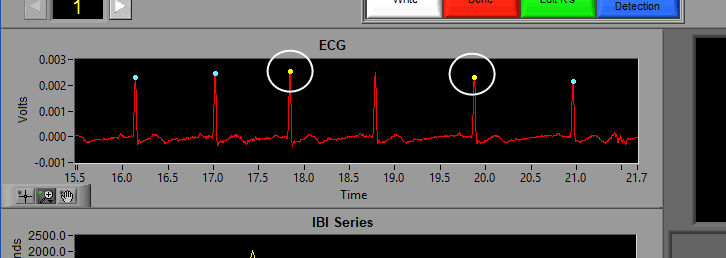
An orange cross around a blue or yellow dot indicates that the beat has been marked as an estimate in the Signal Editor. We will talk about this more in that section of the guide:

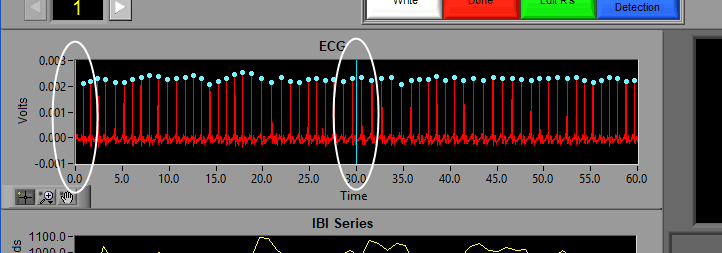
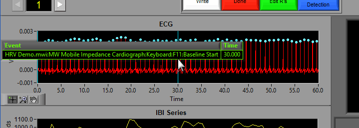
Event Markers
If events are being used for analysis, the locations of any events in the segment will appear as blue vertical lines throughout the segment.
To reveal the name and time of the event, hover the mouse over the vertical line:
Video Position
If videos have been selected for playback, a yellow vertical line indicating the current video position will appear:
Left-click and drag the yellow position line to update the video position accordingly:
Interval Mode
When analyzing in Interval mode, additional grey lines will appear on the graph indicating the intervals used for calculating each of the statistics.
You may notice that the segment time shown does not match the segment time requested when in interval mode. This is because heart rate calculation in smaller intervals requires some knowledge of the beats immediately before and after that interval. The thick grey lines indicate the actual start and end of the segment:
Invert ECG
If your ECG series appears inverted, simply right-click the graph and choose Invert ECG:
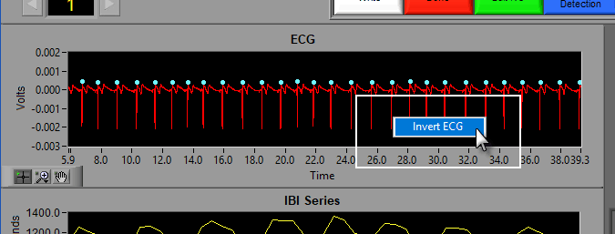
To un-invert the signal, repeat the procedure.
Note: Signal can only be inverted when an edit file is not in use.
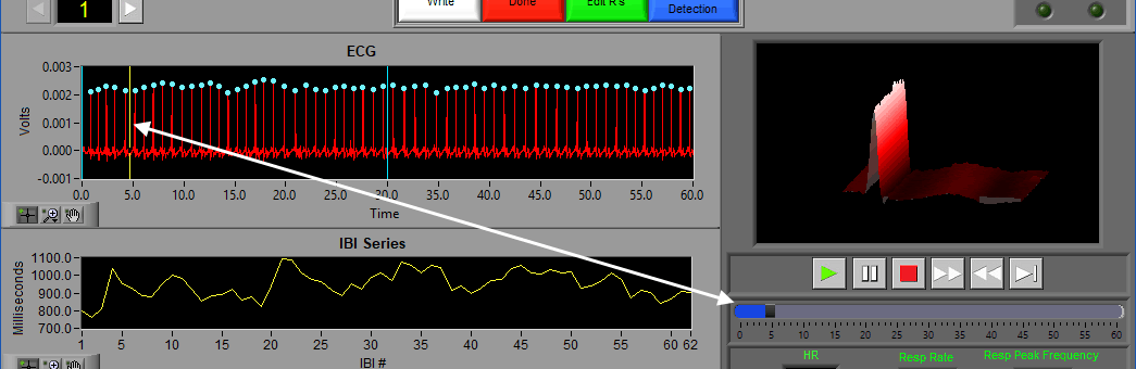
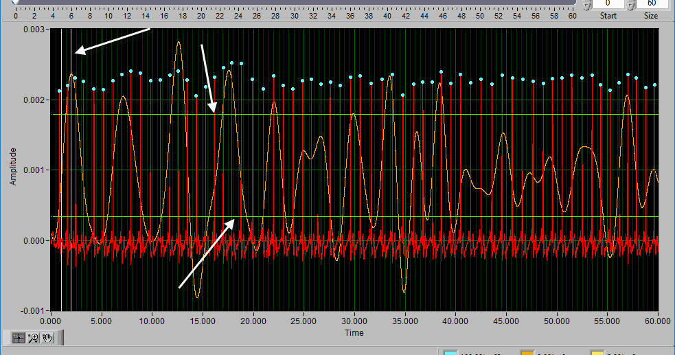
IBI Series
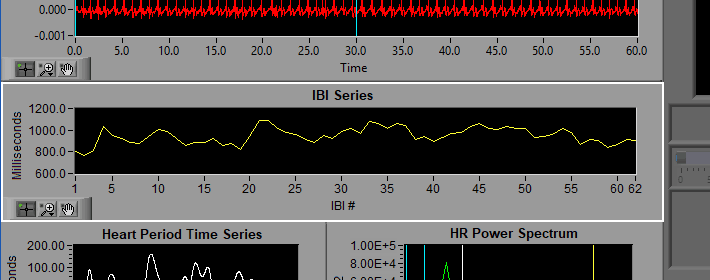
The IBI series is built from the timing between all annotated beats on the ECG series. Notice the X axis is no longer in time, but rather the index of the interbeat interval as detected in ECG. The Y axis indicates the duration of each of these intervals.
Heart Period Time Series
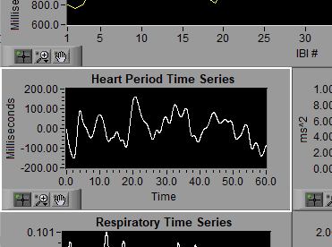
The IBI series is then interpolated and detrended to create the Heart Period Time Series. This is done as an intermediate step to prepare it for frequency-based analysis.
HR Power Spectrum
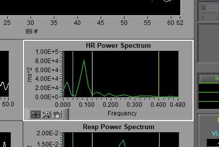
The vertical cursors here indicate the frequency bands as specified on the setup screen. VLF=Blue, LF = White, HF/RSA = Yellow. It is from this information that RSA, an index of high-frequency heart rate variability, is derived.
Respiration Time Series
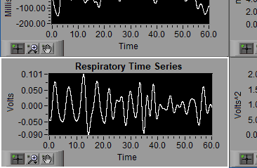
The respiration signal, either directly from a respiration channel in the data file or derived from cardiac impedance.
Resp Power Spectrum

The respiration signal can be passed directly to an FFT for frequency-based analysis. The same bands appear here as in the HR Power Spectrum.
Statistics
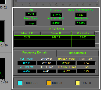
The following statistics are computed:
HR
Heart rate is displayed in beats per minute (BPM)
Resp Rate
Calculated from the peak frequency in the Respiratory Power Spectrum, in breaths per minute
Resp Peak Frequency
Frequency with the most power as detected in the Respiratory Power Spectrum, displayed in Hz. The presence of this frequency in the HF/RSA band is used to validate the RSA statistic. If this peak is located outside of the HF/RSA band, it will turn red to draw your attention to it.

Resp Signal
Indicates the type of signal used to derive the respiration signal, as specified on the setup screen.
Resp Amplitude
Power of the resp peak frequency, in volts2.
Resp Power
Integral of the Resp Power Spectrum, indicative of the total respiratory power.
HRV Stats
The HRV Stats table contains 3 columns, one for each of 3 statistics:
- Mean HR – Average heart rate in beats per minute
- Mean IBI – Average interbeat interval in milliseconds
- # R Peaks – Total number of R peaks identified
When analyzing in Entire mode, there will be a single row representative of the entire segment. If you are using Interval mode, each row will represent statistics for a single interval in the segment.
Frequency-Domain
Statistics derived from the HR Power Spectrum are shown in the Frequency-Domain tab.

For each frequency band (VLF, LF, and HF/RSA), two statistics are calculated
- Power – integral of the signal in the specified frequency band, measured in ms2
- Pk Frequency – frequency within the band with the most spectral power, in Hz.
In addition to these statistics, the following are also computed:
LF/HF Ratio
Ratio of power in the LF and HF/RSA bands.
RSA
Respiratory sinus arrhythmia is a widely used index of high-frequency heart rate variability. It is calculated by taking the natural log of the HF/RSA band power. The RSA statistic will turn red if more than 10% of total beats within a segment are estimated. This is to aid in applying the 10% rule as discussed here.
Time-Domain
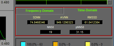
Time domain statistics are primarily derived from the IBI series. Many of these statistics refer to N-N intervals, which is a way of writing normal R-R intervals.
- SDNN – The standard deviation of N-N intervals
- AVNN – Average N-N interval. Should be equal to Mean IBI for the segment
- RMSSD – Root mean square of successive differences. It is calculated by taking the RMS of differences between successive N-N intervals
- NN50 and pNN50
- NN50 represents the number of N-N intervals which differ by more than 50ms from the previous interval, and pNN50 is the proportion of these intervals relative to the total time segment.
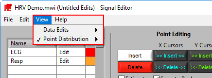
Point Distribution/Data Edits
Using the View menu, the information shown in the bottom right corner of the screen can toggle between the point distribution on the ECG signal and information on the data edits performed on any of the signals in use.
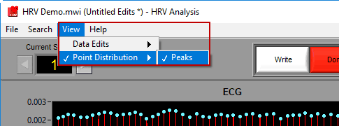
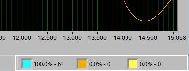
Point Distribution
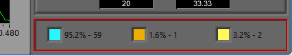
Recall the types of annotations found on the ECG graph. Blue for good R peaks, yellow for artifact peaks, and orange for estimated peaks. The point distribution shows how many of each occur in the given segment and their percentage of the whole. There are some widely accepted rules to follow regarding how many estimate/artifact beats can exist in a segment while still maintaining valid statistics. This display can help in ensuring that these rules aren’t broken.
Data Edits
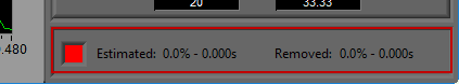
The data edits display shows the amount of the signal (in time and percent of total signal) that has been estimated or removed using the signal editor. This will make more sense as you learn about the signal editor.
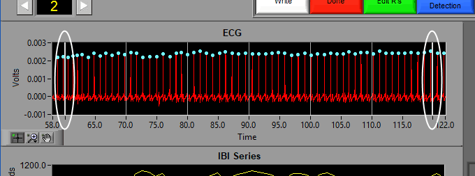
Navigating through segments
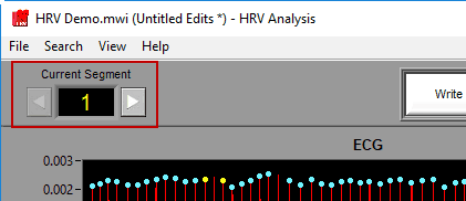
Use the left and right arrow buttons, or the left and right arrow keys on the keyboard to move forward/backward in the file.
To jump to a specific segment quickly, click the current segment number and select a new one from the list.
Advanced Segment Navigation
It is also possible to jump to the next (or previous) segment which meets certain criteria. These searches can take a few moments, so while they are taking place a small popup will appear. End the search at any time by pressing “Cancel”. The following options are available in the Search Menu
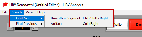
Next/Previous Unwritten Segment
Finds the next/previous segment which has not yet been written to the currently opened output file. This search can also be run by pressing Ctrl+Shift+Left Arrow or Ctrl+Shift+Right Arrow.
Next/Previous Artifact
Locates the next/previous segment which contains an R peak that has been identified as an artifact. This search can also be run by holding Ctrl and pressing the left or right arrow key.
Writing data to the output file
Statistics and setup information can be written to an Excel spreadsheet (.xlsx) for import into study-level statistics applications, or for offline processing. Output files are automatically saved after each write.
Note: Excel does not need to be installed on the computer to successfully write output files
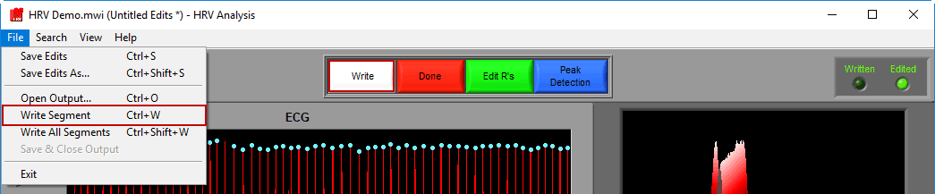
To write a segment, either press the white Write button, navigate to File>>Write Segment, or use the Ctrl+W hotkey.
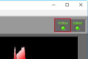
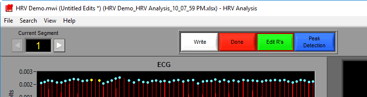
When a segment has been written to the current output file, the Written light will be illuminated in the upper right-hand corner
If a segment has been edited since it was last written to the output file, the statistics in the output will no longer match what is on the analysis screen. To indicate this, the Written light will turn red
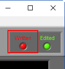
Be sure to re-write the segment in this case so that the output file contains the desired statistics.
Creating a new output file
To begin writing an output file, press the Write button on the toolbar. You will be prompted to select a location and filename for the output file:
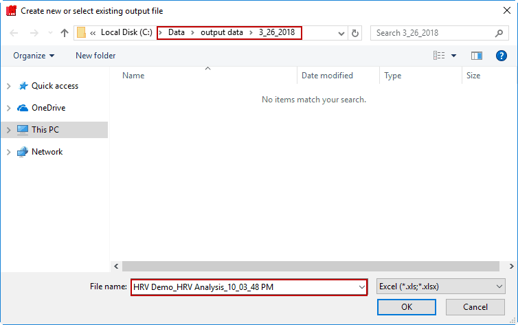
The default name is:
Data file name_HRV Analysis_Current Time.xlsx
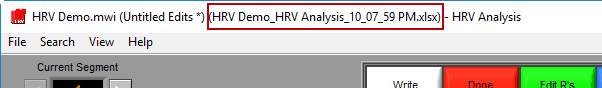
You are welcome to change this based on your needs. Once an output file is opened, you will see its filename appear in the title bar.
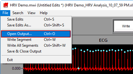
Opening an existing output file
To append a segment to an existing output file, either select an existing output file when prompted after pressing Write or go to File>>Open Output (or press Ctrl+O). Opening an output file will automatically detect which segments have already been written.
Note: This should only be done when analyzing the same data file using the same events & modes settings in the same analysis application. Appending to output files which were written with a different segmentation will have undesirable effects since the segment numbers overlap.
When opening an existing output file, segments which have been written to that output file but could differ from the statistics currently shown on the analysis screen will cause Written light to turn yellow
If you believe your segments/edits have changed since the output file was last written, you should re-write the segment.
Saving and closing an output file
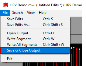
Output files are automatically saved after each segment write. They are also automatically closed when the Analysis screen is closed, but to close the output file manually go to File>>Save and Close Output.
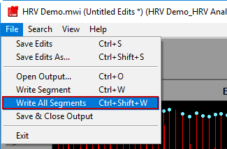
Write All Segments
A shortcut to writing all segments to the output file can be found in File>>Write All Segments, or by pressing Ctrl+Shift+W on the keyboard. This mode will automatically iterate through all segments, writing each of them to Excel. This can take a few minutes depending on how many segments are being analyzed. You can press cancel on the popup at any time to end the process.
Note: this can be a time-saving tool and can give you an idea of what statistics have been calculated throughout the segments, but it is not a substitute for careful examination of data on a segment by segment basis. Be careful that this tool is not abused.
Data Editing
Often times data is not perfect – but that does not mean it isn’t salvageable with a bit of editing. To launch the signal editor, press the Edit R’s button in the toolbar.
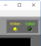
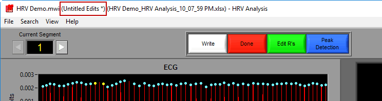
If an edit file is currently being used, you will see the filename appear in the title bar. If the current segment has been edited, Edited will be illuminated in the upper right-hand corner.
Saving the edit file
A ‘*’ next to the edit file name means changes have been made but not yet saved to the file.
To save the changes to the edit file, go to File>>Save Edits or press Ctrl+S. If a new edit file is being created, a prompt will appear asking you to specify a name and location for the file. By default, edit files are saved in a subdirectory of the same directory as the data with the following naming convention:
/Edit Files/Data file name.edh2
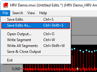
To save a copy of the currently opened edit file, go to File>>Save Edits As… or press Ctrl+Shift+S.
Video Playback
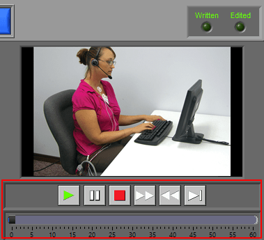
Video playback controls are found below the single video window. All standard video controls are here, including slow video playback. To jump to a specific time in the video (within the current segment), drag the time slider to the desired position. The yellow position in the ECG graph will update accordingly.
If more than one video has been selected for playback, multiple videos will be shown in a separate window.
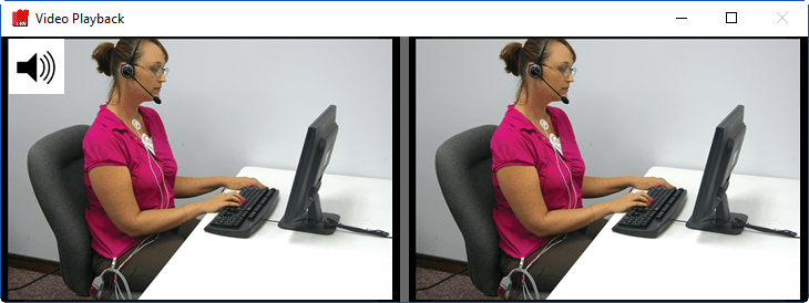
Only one video will play its audio content at a time. This is indicated by a speaker symbol embedded in the video. To cycle through the audio on different videos, left-click the desired video.
Exiting the Analysis Screen
To close the analysis screen, press Done in the toolbar, go to File>>Exit, or simply close the window.

If any edits have been made but not saved, you will be prompted to save or discard those changes prior to closing the screen.
Continuous Analysis
When analyzing in Continuous mode, the analysis screen will look quite different from normal analysis:
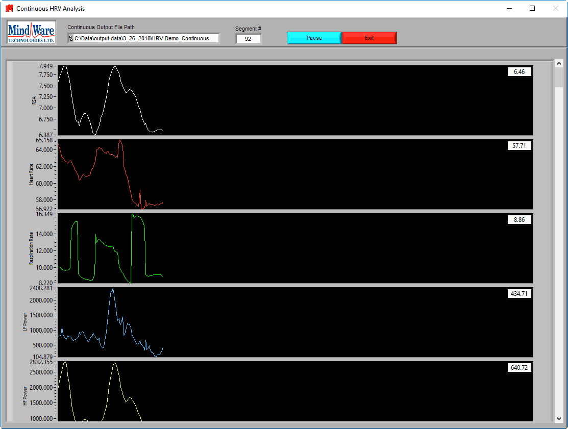
Statistics will be plotted on the graphs as they are calculated for each instance of the moving buffer. Press Pause at any time to temporarily stop the analysis.
Continuous statistics are written to a tab-delimited text file, which you will be prompted to specify before analysis begins. By default, it is named:
Data-file-name_Continuous HRV Analysis_Current Time.txt
When the entire file has been analyzed, press Exit to return to the Setup screen.
Signal Editor
No matter how hard you try, your data set will not be perfect. Electrodes, lead wires, physical movement, and much more can lead to incorrectly detected/missed R peaks on the ECG signal, or impossible fluctuations in respiration. The signal editor is used to correct these mistakes. It is quite likely that the editor will be where you spend the majority of your time in the HRV application.
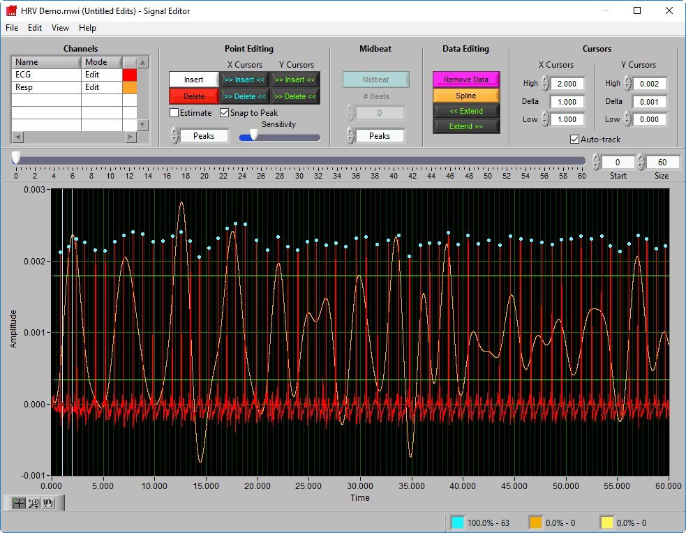
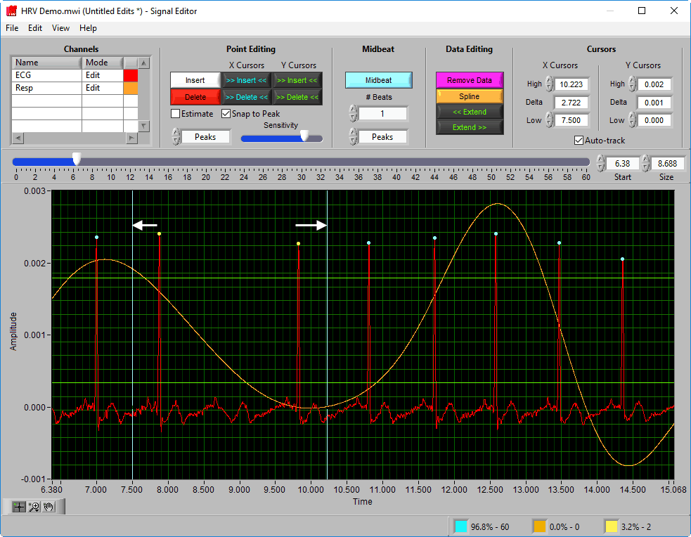
Data Graph

The data graph is loaded with the same data used on the analysis screen for the current segment. LIke the analysis screen, the ECG signal has detected R peaks annotated in a few colors: a blue dot for a “good” beat, a yellow dot for a beat that failed artifact detection algorithms, and an orange cross for an estimated beat.
To gain some insight as to why a peak is marked a certain way, left-click on it in the graph.
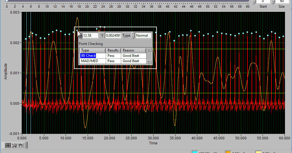
If multiple signals are used for analysis, you will notice they appear overlayed on the graph. All signals used for analysis can be edited. There are some options for modifying which channels are edited and in what way using the Channels options in the toolbar.
Additionally, there are two vertical blue cursors and two horizontal green cursors on the graph. They are referred to as X cursors and Y cursors, respectively, after the axis upon which they move. These are used for several of the tools in the editor to define regions of interest. To move them, left-click and drag them to the desired location.
Navigating through the data
Editing requires a bit of precision with the mouse, and often times this is made much easier by zooming into sections of the data that require attention. The same graph tools from the analysis screen are available in the editor for various types of zooming. See this article for more information on how to use these tools.
Pressing the space bar will automatically cycle through the tools.
To scroll through the data once zoomed in, use the scroll bar at the top of the graph. You can also adjust the window size to precisely change the amount of data on the screen.
To scroll through the data second by second, press the left and right arrow keys on the keyboard.
Point Distribution/Data Edits
Remember this information from the analysis screen? It is also found in the editor, where it is updated in real time as edits are made. This can be very useful for ensuring that you aren’t exceeding any editing limitations
Like on the analysis screen, the View menu is used to toggle between the types of information shown here
Toolbar
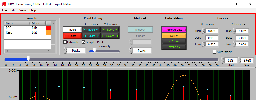
Channels

This list contains all channels that are being edited, along with two characteristics – Mode and Color.
There are 3 modes for each channel – Edit, View, and Hide.
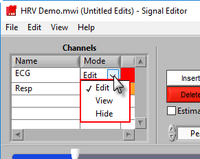
In Edit mode, various editing actions will affect the channel when they are performed. When a channel is in View mode, that channel is only shown in the graph for reference, and will not be affected by editing. Finally, Hide mode will remove the channel from the graph.
To change the color of the signal in the graph, left-click on the color column and select a new one from the window.

Point Editing
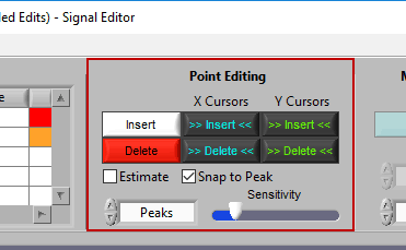
These are the tools you will use for inserting/deleting R peaks on the ECG signal.
Types of points

As we have discussed a few times so far, there are a few different ways points can be classified. The insert tool is almost always used to insert (or at least attempt to insert) a good R peak that is actually visible on the signal. To do this, ensure that Estimate is unchecked. If you do want to insert a peak as an estimate, simply check this box.
Insert
To insert a peak, first activate the insert tool by left-clicking on the Insert button, or press I on the keyboard.
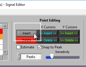
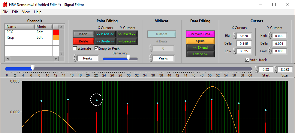
When you move your mouse into the graph, you will notice that the mouse cursor has been replaced by a white dotted circle:
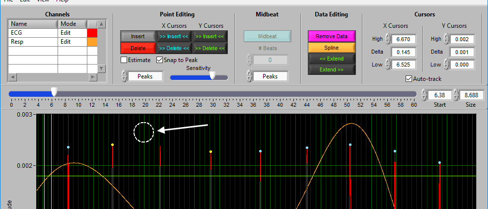
This circle defines the region on the graph where you want to insert an R peak. The diameter of this circle can be increased/decreased by using the Sensitivity slider or with the mouse scroll wheel.

Once a portion of the signal has been identified as the R peak you wish to insert, left-click to insert it.
To deselect the insert tool, either click the button again or press the Escape key.
Delete
The delete tool works similarly to insert. To select it, press the Delete button or D on the keyboard
This time, the dotted circle on the graph is red. Identify the region where you want to delete an R peak, and left click to delete it.

Note: All peaks found within the region will be deleted, so be sure to adjust the sensitivity accordingly.
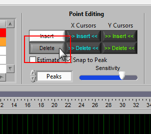
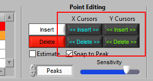
Using Cursors to Insert/Delete Multiple Points
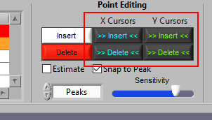
It is also possible to insert/delete many points at once by using the X/Y cursors. Each of these buttons has 4 different modes. By default, they will operate on the signal between the cursors, as indicated by the >> << symbols.
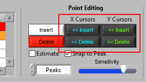
Hold Ctrl to perform the action before the low X cursor or below the low Y cursor:
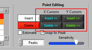
Hold Shift to look after the high X cursor or above the high Y cursor:
Or hold Ctrl+Shift to look outside the cursors in both directions:
Let’s take a look at some examples of when this would be used.
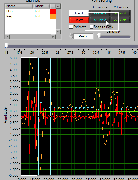
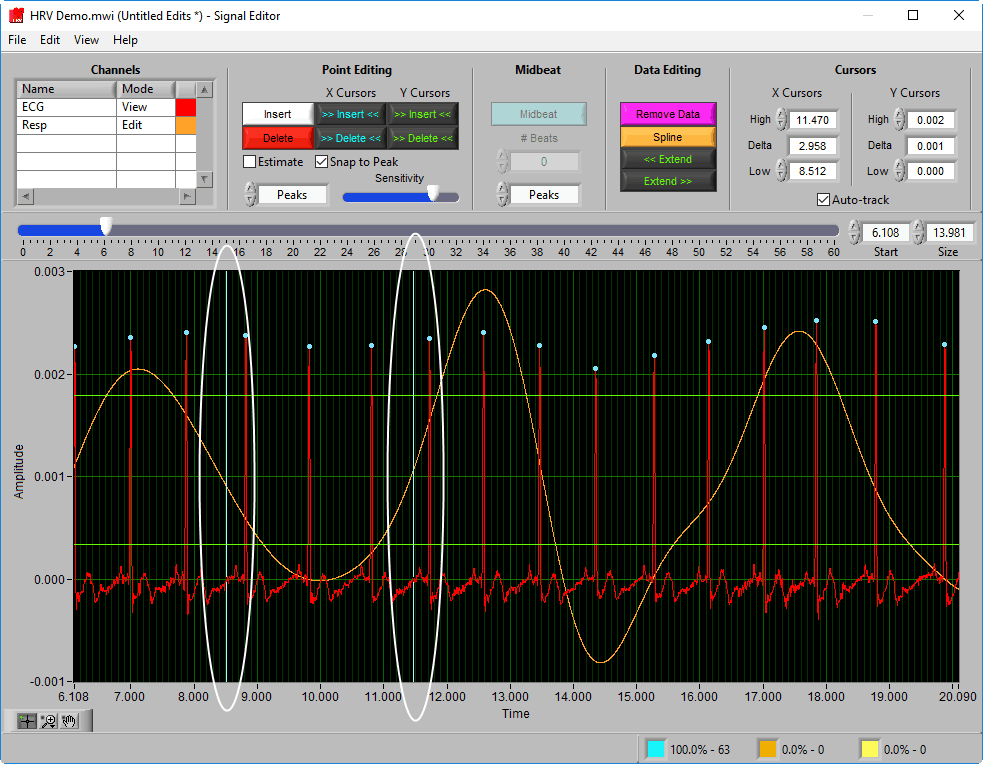
Delete All using X cursors
Suppose there is a section of noise which resulted in many incorrectly identified R peaks.
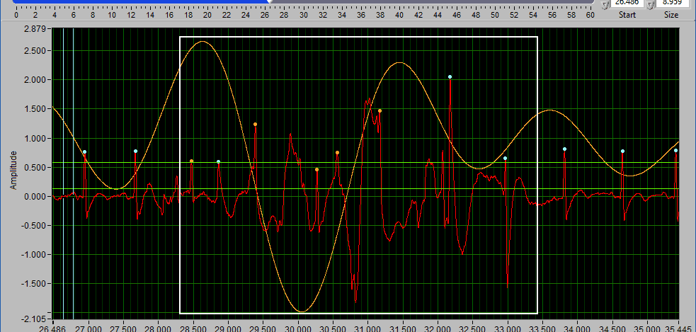
To delete all of these, drag the X cursors on either side of the noise, and press Delete All:
Due to the need for a 30-second contiguous R peak series when calculating RSA, points will need to be identified or estimated when making the above edit.
Because of this rule, a common use for the Delete All tool would be to remove all R peaks from the beginning/end of a segment. Do this by dragging the low X cursor to the right of the noise (when removing from the beginning):
Hold Ctrl and press the Delete All button to remove the artifact peaks
Inserting All using X cursors
When a portion of ECG has many R peaks visually, but none have been marked:
Drag the cursors around that section and press Insert All to insert them.
Note: This runs the same peak detection algorithm used to identify the R peaks in the first place.
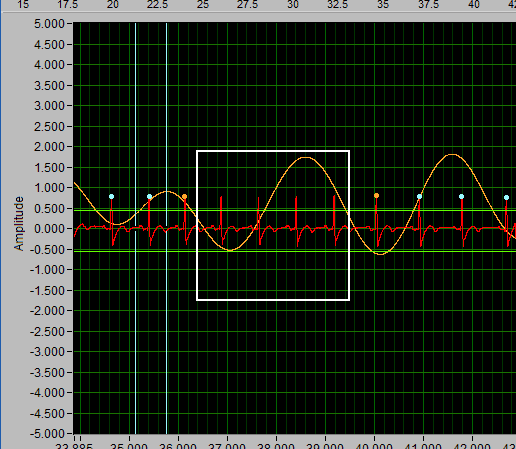
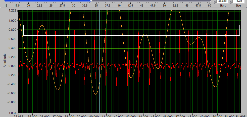
Deleting all using Y cursors
This can be a useful function when the ECG morphology is such that components other than the R peak are being misidentified as the R peak.

Simply drag the cursors to include the erroneous peaks, but exclude the proper ones, and press Delete All.
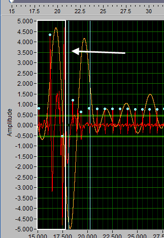
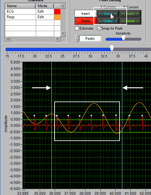
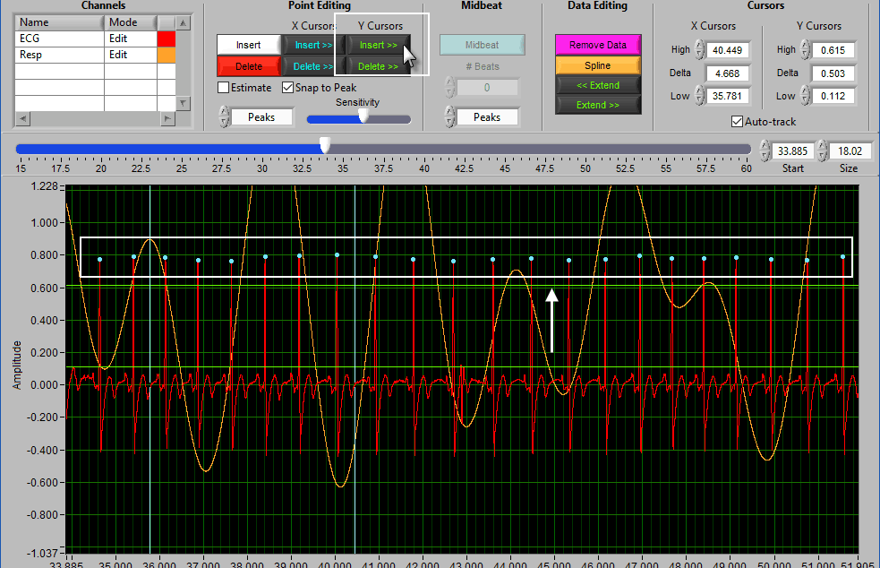
Insert all using Y cursors
This action works similarly to the threshold-based peak detection available from the Setup screen, except you can view the relationship between the threshold and the signal to only include the proper peaks.
A common technique may be to insert all peaks above the high Y cursor. As before, drag the high cursor so it is below most of of the correct peaks:
And press Insert All while holding Shift:
Midbeat
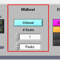
This function is unique to the HRV editor and is used to estimate the location of an R peak when one is not clearly visible.
To insert one or more midbeats, drag the X cursors so that they fall outside two known good beats:
Based on the time between these beats relative to the expected time based on the rest of the segment, the editor will identify how many beats should be inserted to restore proper timing.
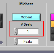
This value can be overridden, but it is a good idea to try the suggested number of beats first and adjust as needed. To insert the midbeat(s), press the Midbeat button.
Since midbeats are not placed on actual R peaks (or even on the ECG waveform for that matter), they will always be classified as estimates.
Note: Inserting too many midbeats at once may affect the validity of HRV statistics. Use with caution. For more information, see this blog post.
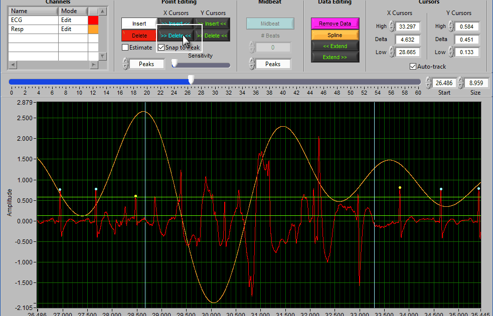
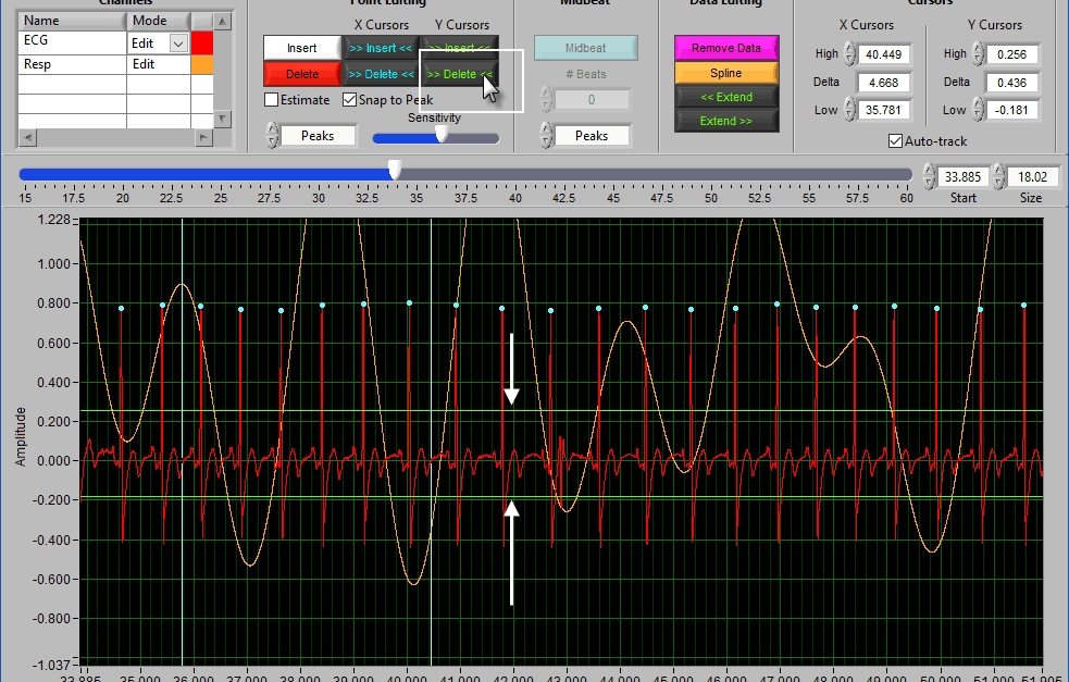
Data Editing
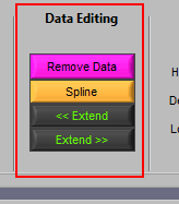
Where point editing tools affect the annotations on the signal, data editing tools affect the signal itself. Each of these tools makes use of the X cursors for defining the affected area of the signal(s).
Note: In HRV, these tools are more useful for editing the respiration waveform than the ECG waveform. When editing ECG, it is considered best practice to remove the peaks rather than modify the waveform itself. To edit the respiration signal independently, ensure that the ECG channel is set to View mode
Remove
The Remove action sets a portion of the waveform to 0. To remove a portion of the signal, drag the X cursors to the appropriate locations and press Remove:
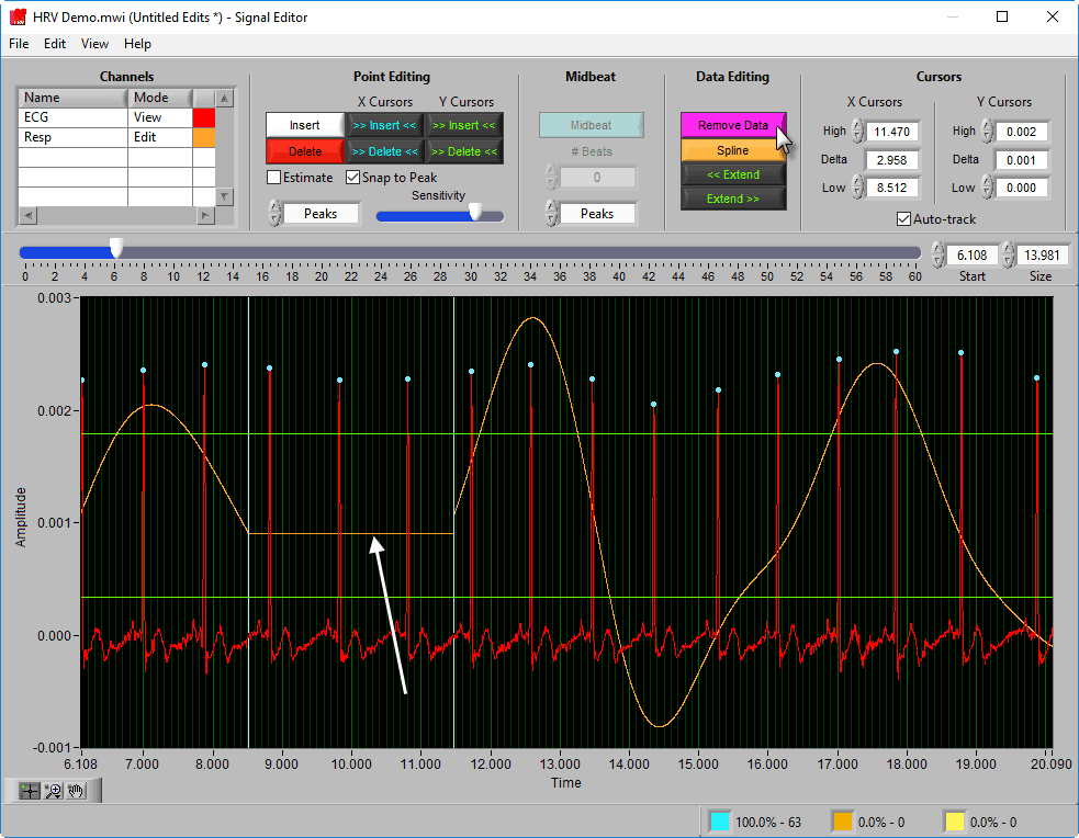
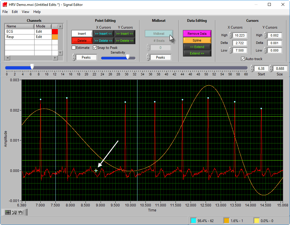
Spline
Splining is useful when signal amplitude must be maintained. Like above, adjust the X cursors to the area you want to estimate, and press Spline:

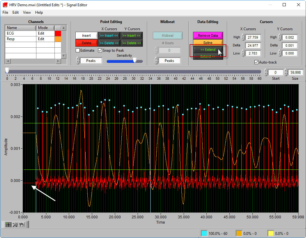
Extend
Extend allows you to preserve the signal amplitude while removing data from the beginning/end of the segment. << Extend uses the leftmost cursor position and extends that data value to the beginning of the segment.
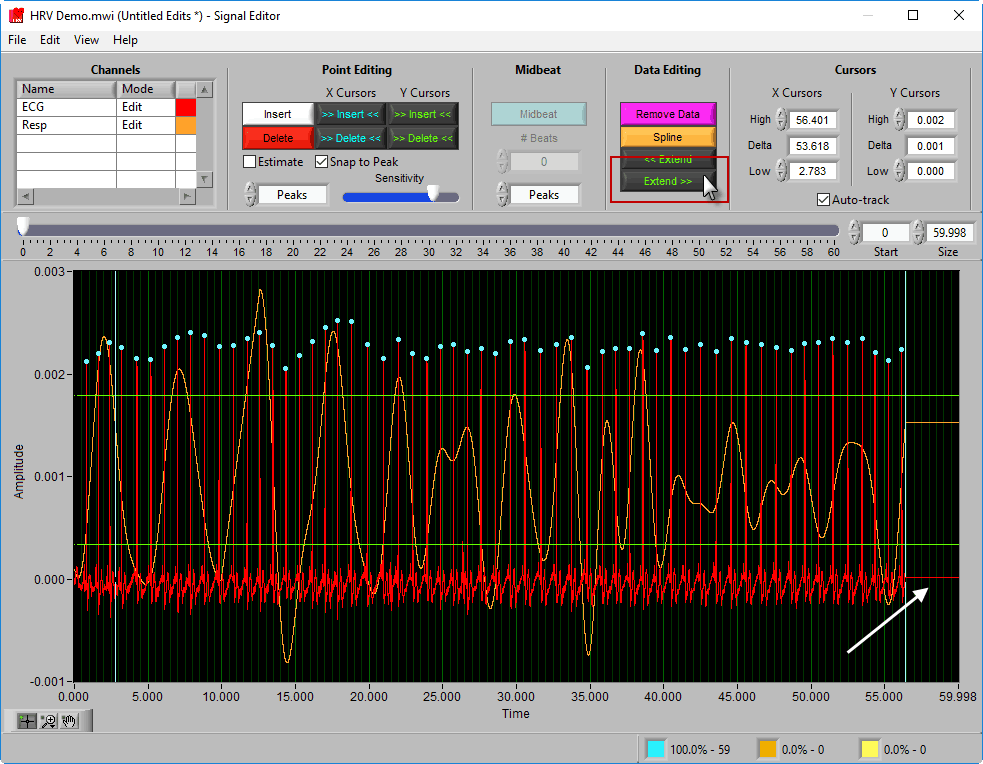
Extend >> uses the rightmost cursor position and extends that data value to the end of the segment.
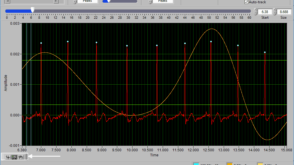
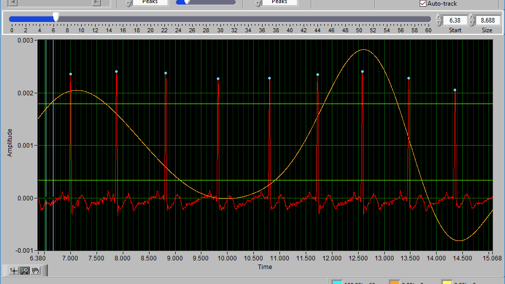
Cursors
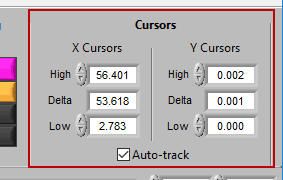
We’ve been talking about cursors extensively throughout this section, and as they are moved the values in this section of the toolbar are updated. You can also specify exactly where a cursor is placed by modifying each position manually.
When Auto-Track is enabled, cursor locations will automatically be updated when scrolling/zooming into data. This is useful to ensure the cursor doesn’t end up out of view. When unchecked, cursors will retain their position regardless of scrolling/zooming.
Some Additional Functions
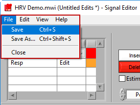
Saving the edit file
The edit file can be saved in the signal editor as you are performing edits. To do this, go to File>>Save or press Ctrl+S. To save a copy of the current edit file, go to File>>Save As… or press Ctrl+Shift+S.
Undo/Redo
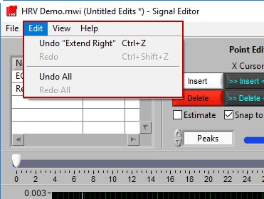
Don’t like an edit you just made? Or the last three edits? Go to Edit>>Undo or press Ctrl+Z to revert back to before that edit. The description in the edit menu gives some insight into the action that will be reversed.
Changed your mind again? Go to Edit>>Redo or press Ctrl+Shift+Z to redo the previously undone action.
Undo/Redo All
Don’t like any of the edits you have performed in this editing session? Go to Edit>>Undo All to undo all changes made to the signals since the editor has been open. Or use Edit>>Redo All to re-apply anything you may have undone. This does not affect edits performed in prior editing sessions.
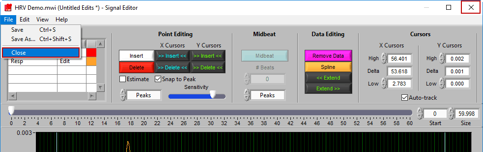
Returning to analysis
When you are finished editing, go to File>>Close or close the window to return to the analysis screen:
Peak Detection

The peak detection window allows you to tweak the peak detection settings on a segment-by-segment basis. This can be useful when there are significant changes in signal morphology throughout the data file. These settings should look familiar – they are the same as what was found on the Setup screen.
Conclusion
If you are eager to learn more, please visit our blog for deep dives into the scientific aspects of the applications, or our knowledge base for more technical information.
Thank you for taking the time reading this manual, and we wish you the best of luck in your research endeavors!