Last time we introduced the following depiction of the dZ/dt signal:

What we are looking at here is a single cycle of dZ/dt. In the IMP Analysis application, we distill a series of cardiac cycles down to a single average cycle for a given time period. It is from this average waveform that we identify the key signal landmarks and calculate related statistics. To do this, we employ a technique called ensemble averaging.
Ensemble Average
To help explain the ensemble averaging process, we need to also talk about the ECG signal, which is required to analyze cardiac impedance data anyway. Lets add a single cycle of ECG data to the previous depiction of dZ/dt:
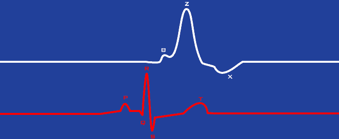
The mechanical activation of the heart (dZ/dt) will always be preceded by the electrical activation of the heart identified by the QRS complex of the ECG signal. Rather than identifying landmarks on the dZ/dt waveform cycle by cycle in the IMP Analysis application, only the R peak on the ECG series is identified. Using this R peak as an anchor, a section of data from both ECG and dZ/dt is extracted. These extracted portions are averaged over the course of the segment of time being analyzed, producing an average representation of the relationship between ECG and dZ/dt for that segment. Essentially, the ensemble average is produced by lining up all of the identified R peaks on top of each other and then averaging the overlapping signals.
Note: Only “good” (non-artifact) R peaks are used to build the ensemble average. This ensures that only quality representations of cardiac cycles are included.
The amount of data extracted surrounding each R peak is chosen on the IMP Calibration Settings tab on the Setup screen:
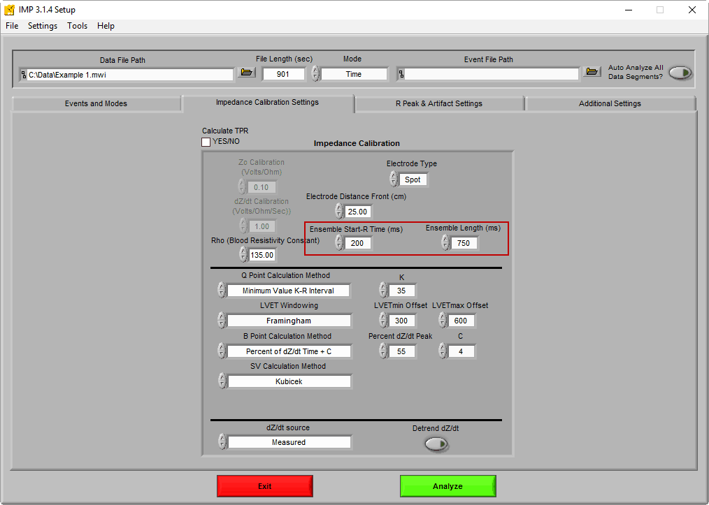
By default, the ensemble window consists of data starting 200 milliseconds before the R peak of ECG and 750 milliseconds total. This window ensures that all important landmarks on both ECG and dZ/dt will fall within that time frame for the typical heart rate.
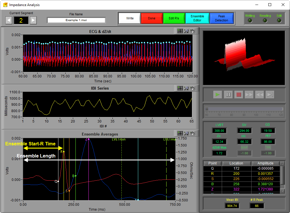
When viewing the analysis screen in the IMP Analysis application, the Ensemble Average plot can be found at the bottom of the screen.
It is possible at certain heart rates that the default windowing may need to be modified. For example, if you are working with higher heart rates, you will see a 2nd ECG and dZ/dt cycle within the ensemble window

The algorithms for identifying landmarks in the ensemble average are designed to ignore this extra cycle, but it is ideal to adjust the ensemble window to focus on a single cardiac cycle.
At the opposite end of the spectrum, it is possible to view too short of an ensemble window, cutting off the end of the dZ/dt cycle. This could result in incorrect identification of the X point, which is an important landmark for calculating LVET.
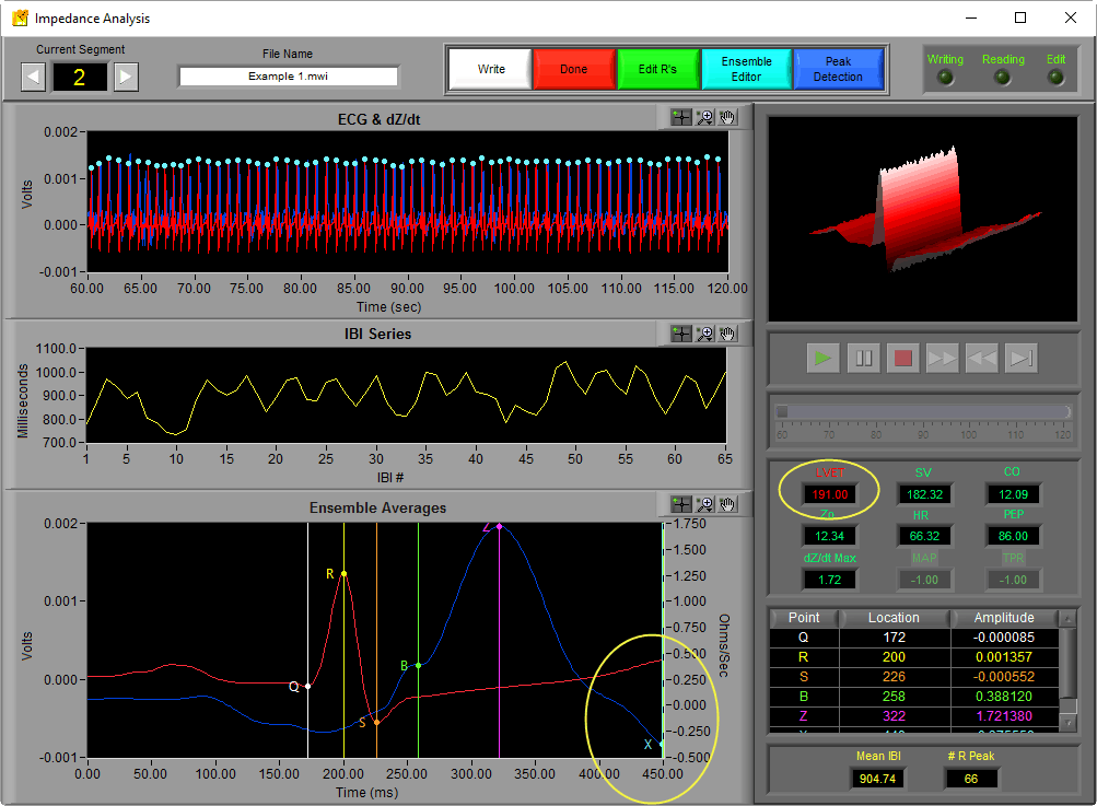
We’ll touch more on this later, but in cases where this happens, the LVET statistic will turn red, meaning the X point placement was estimated.
For best results, you should set the ensemble window to handle the slowest heart rate in your data file, and on segments where a 2nd cardiac cycle appears, simply ensure that no landmarks are being identified on it.
The default values usually work pretty well.
Next time…
Next time we will talk more about the landmarks identified on the dZ/dt waveform and the algorithms used for identifying them.