Select analysis version to view the applicable content:
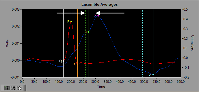
Last time we talked about how an entire segment of data is distilled down to an average representation of the cardiac cycle using ensemble averaging. Using the ensemble average, three landmarks are identified on the dZ/dt waveform: B, Z, and X. All three of these points are important to identify correctly as they are used to calculate significant systolic time intervals (PEP, LVET) as well as stroke volume and cardiac output. This article will go over the various algorithms available to automatically identify these landmarks and how to best use them.

B Point
The B point is identified as the notch/upstroke that occurs on the dZ/dt waveform as it rises to its maximum. Physiologically, it corresponds to the opening of the aortic valve.

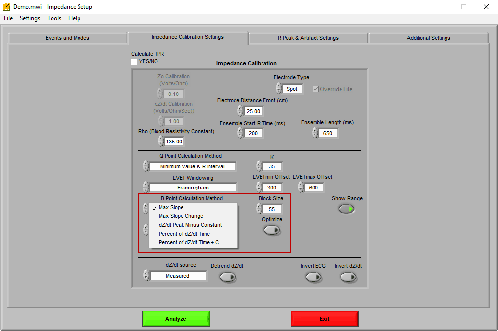
There is no single accepted method for finding the B point, as the best method can depend on signal quality. The MindWare IMP Analysis application contains several algorithms for automatically identifying the B point on the dZ/dt ensemble average, located on the Impedance Calibration Settings tab.
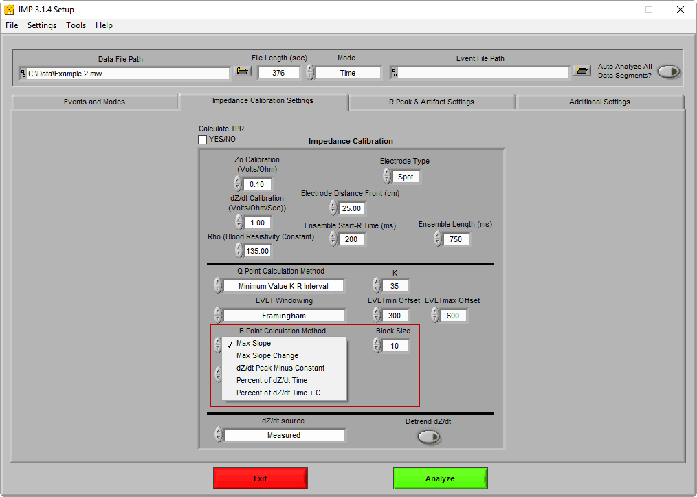
The following two methods are recommended when the B notch/upstroke is visible:
Max Slope – Also known as the 2nd derivative method. The B point is identified as the inflection point on the 2nd derivative of Zo between the R peak of ECG and the Z point of dZ/dt. The Block Size is the span of points that the slope is found between. Increasing this value is useful for noise rejection. See this paper for more info.
Max Slope Change – Also known as the 3rd derivative method. The B point is identified as the peak of the 3rd derivative of Zo between the R peak of ECG and the Z point of dZ/dt. Again, the Block Size is the span of points that the slope is found between. See this paper for more info.
The next three methods are recommended when the B notch/upstroke is not visible:
dZ/dt Peak Minus Constant – Places B point at a constant millisecond value prior to Z.
Percent of dZ/dt Time – Places B point at a certain percentage of the R-Z interval. See this paper for more info.
Percent of dZ/dt Time + C – Uses the same technique as the previous method, but adds a constant millisecond value C to the placement time. See above paper for more info. Per the conclusions drawn in the paper, C is typically set to “4”.
The Show Range button toggles two additional cursors on the Ensemble Average graph which indicate the most likely location of the B point based on PEP values gathered from a large, diverse population. This range does not affect the placement of the B point based on the algorithm chosen but can act as a guideline for confirming the validity of the placement.
Z Point
The Z point, sometimes referred to as the C point or dZ/dtMAX, is the maximum point on the dZ/dt waveform between the B point and X point.

It is identified by simply looking for the maximum value between the B point and the soonest possible location of the X point (which we will discuss further in a moment).
X Point
The X point is the trough following the Z point within a known time span, which corresponds to the closing of the aortic valve.

The location of the X point can be particularly difficult to identify due to the signal morphology and the typical downward drift of dZ/dt at the end of the cardiac cycle. To help narrow down the area in which the X point can be identified, we define an LVET Window in which to look. Now would be a good time to define LVET as the Left Ventricular Ejection Time defined by the time interval between the B point and X point, or the opening and closing of the aortic valve.

There are 2 LVET Windowing options in the application:
Framingham
Here, we need to bring the ECG signal back in the mix. The Framingham method uses the large, diverse data set from the Framingham Heart Study to estimate the QT interval on ECG as a function of heart rate. We know that the X point will always fall after the T wave, so by identifying the location of T, we can determine our LVETmin. Using the equation
LVETmin = LVETmin Offset – 0.154 * (1 – RR)
where
LVETmin Offset = Shortest possible LVET. Default value is 300 for normal QT interval
RR = Average R-R interval in milliseconds for segment. Also referred to as the inter-beat interval.
we can define the minimum possible location of X.
Next we need to identify the maximum possible location for X. Again by using a known large data set and correcting for heart rate, we can determine how long a normal LVET can be. Using the following equation
LVETmax = (LVETmax Offset – 2.5 * HR) + 0.55RZ + 4.5
where
LVETmax Offset = Longest possible LVET. Default value is 600 for normal population
HR = Heart rate for segment
RZ = Time interval between R peak of ECG and Z point on dZ/dt
we can determine the maximum possible location of X. The lowest trough within this LVET window is considered to be the X point.
Estimating X
The Framingham model is not perfect, and signal morphology of dZ/dt is not consistent. Due to this there is a need to be able to estimate the X point location in the absence of a trough in the LVET window, or if the dZ/dt signal is still trending downward at the end of the window. To do this, we use a comprehensive data set to place the X point at the average LVET as a function of heart rate with the following equation:
LVET = 473 – 2 * HR
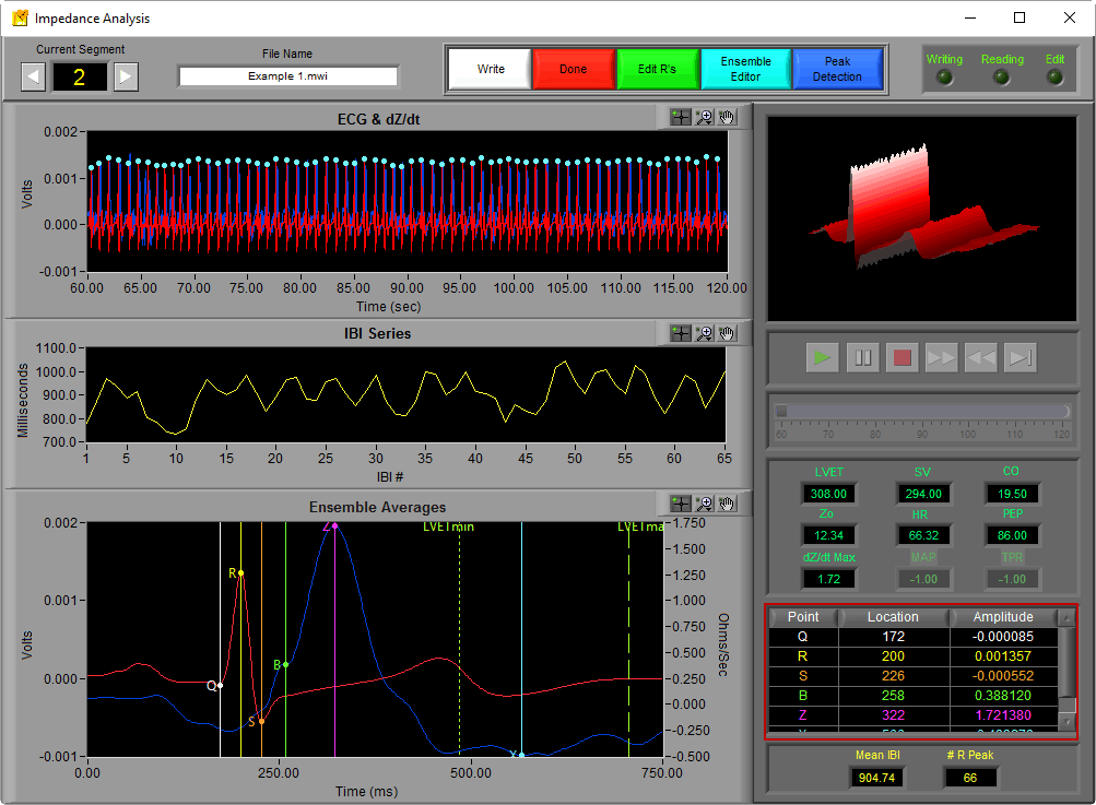
We are getting a little ahead of ourselves, but when the X point is estimated, the LVET statistic on the IMP analysis screen will turn red.

RR Minus Constant
This is a more simple method for identifying the X point. It simply looks for a trough between the Z point of dZ/dt and the average R-R interval minus some constant value. This method can be useful if the study population is known to have abnormal cardiac timing, or if you are working with non-human subjects.
Helpful Hints
The exact locations of each of these points are not only exported in the output file, but also located in the ensemble points table on the analysis screen:
Some good starting points for locating the B and X points are:
- B Point Calculation Method:
- If notch/upstroke in dZ/dt is visible, select Max Slope Change with a Block Size of 10
- If not visible, select Percent of dZ/dt Time + C with Percent dZ/dt Peak = 55 and C = 4
- LVET Windowing (used to determine the X point)
- If working with “normal” human population, select Framingham with LVETmin Offset = 300 and LVETmax Offset = 600
- Otherwise, use RR Minus Constant or adjust your parameters to match physiological timing norms for your population
Next time we will look at how these points are used to obtain important systolic timing intervals, among other statistics of interest.